6  Convert tree-level metrics to plot-scale

In this target we aggregate the individual tree-level data to the plot-scale, providing estimates for the total Above Ground Carbon (AGC) and merchantable Volume (MV) for every plot.

The below table (Table 6.1) presents the plot-level data for both sampling years and includes a variety of aggregated forest plot metrics.

Table 6.1: Plot-level statistics for all kuamut forest plots.

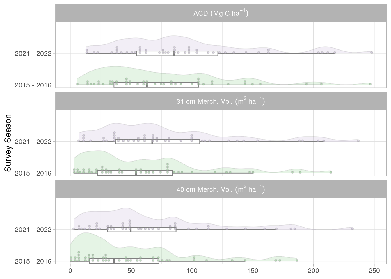
These plot-level values are vital for the further steps in the pipeline, allowing us to develop a strong empirical understanding of forest dynamics at these plots between sampling periods. Figure 6.1 presents these data for three different metrics; Aboveground Carbon Density (ACD), and Merchantable Volume for trees with a DBH > 31cm and 40cm. In All cases we see mean growth when considering the full distribution of plots.

Figure 6.1: Above Ground Carbon density for plots from the two sampling seasons.

6.1 Inspect Plot level growth rates

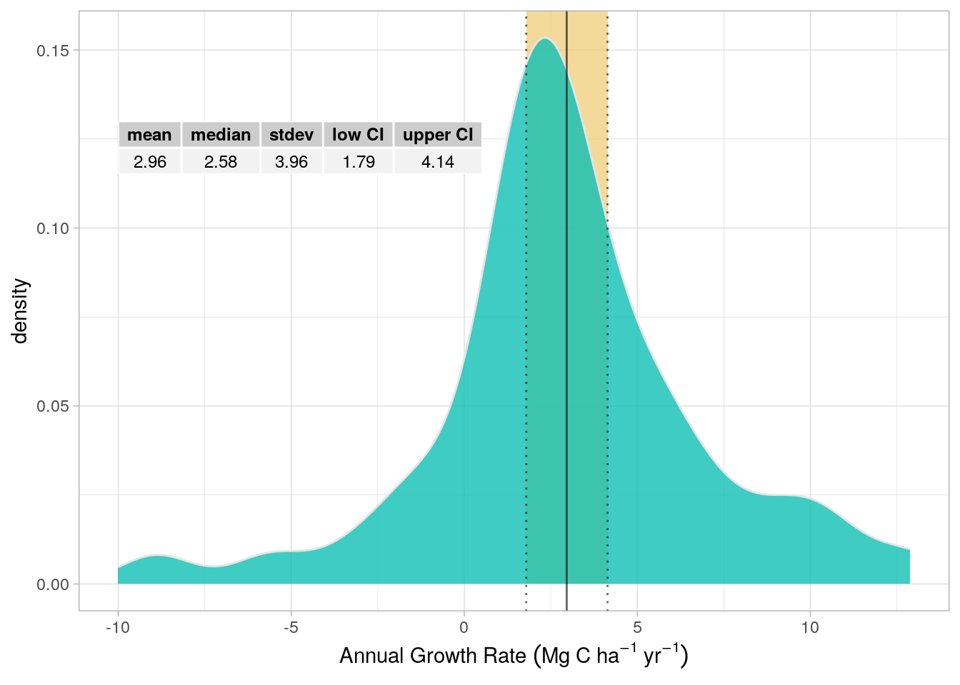
It is also possible, with these plot level data, to investigate plot-level growth, and estimate a mean growth rate for the plot network, as presented in Figure 6.2. The purpose of this target is to investigate the growth rate that was recorded in forest plots between the field surveys in 2016 and 2022. These growth rates are not used directly for the carbon emissions calculations but provide a means by which to evaluate the modelled growth rates which were used for the final calculations and are presented in Chapter 17.

Figure 6.2: Annual Biomass Growth Rates measured at Forest Plots between 2016 and 2022. Green shaded area shows the density distribution of the measured growth rates. Orange shading (and corresponding doted lines show the 95% confidence intervals (CI) around the mean growth rate (solid vertical line)

6.2 Code

#' Convert Tree level metrics to plot level.
#'
#' This function computes Plot level estimates from Tree-level estimates of
#' biomass, volume and carbon  (see Kuamut_TreeAllometrics.R)
#'
#' @param tree_metrics_csv csv path exported from `KuamutTreeLevelMetrics()`
#' @param plots_correct_area_spat
#' @param BCEF_R Biomass Conversion Expansion Factor default is 1.89. IPCC
#' default is 1.67.
#'
#' @details
#' Fits with Approved VCS Methodology VM0010 Version 1.2, 27 March 2013,
#' Sectoral Scope 14 Methodology for Improved Forest Management: Conversion from
#' Logged to Protected Forest
#'
#' 8.1.1 Calculation of carbon stocks in commercial timber volumes
#' This section calculates CHB,j,i|BSL, the mean carbon stock in total harvested
#' biomass in tC<U+00B7>ha-1 and CEX,j,i|BSL, the mean carbon stock in extracted
#' timber (merchantable timber that leaves the forest) in tC<U+00B7>ha-1.
#' CHB =the mean carbon stock in total harvested biomass
#' CEX =the mean carbon stock in extracted timber (merchantable timber that
#' leaves the forest)
#'
#' NOTE: methodology actually says CF = 0.5 - which would be better for us.
#'
#' Load Tree-level dataset with AGB, carbon and volume estimates for each tree
#' Created in `Kuamut_TreeAllometrics.R`. Our biomass equations estimate the
#' entire aboveground biomass of the tree converting to volume by only dividing
#' by density therefore estimates too much timber volume. For this reason we
#' add the additional very conservative step of diving through by Biomass
#' Conversion Expansion Factor BCEF_R
#'
#' @return A list with two file paths named: plot_species_list and
#' plot_level_values.
tree_to_plot <- function(tree_metrics_csv, plots_correct_area_spat,
                         BCEF_R = 1.89, .site = "kuamut") {
  if (is.character(tree_metrics_csv)) {
    kuamut <- readr::read_csv(tree_metrics_csv, show_col_types = FALSE)
  } else {
    kuamut <- tree_metrics_csv
  }

  kuamut <- kuamut |>
    mutate(
      TimbVol = AGB / BCEF_R,
      PlotNo = as.integer(PlotNo)
    )

  # Make data table of all known species
  kuamutSp <- kuamut |>
    dplyr::filter(!is.na(Family)) |>
    mutate(
      Species = case_when(
        is.na(Species) ~ "sp",
        TRUE ~ Species
      ),
      Names = paste(Family, Genus, Species)
    ) |>
    pull(Names) |>
    as.factor() |>
    levels() |>
    data.frame() |>
    tidyr::separate(1, c("Family", "Genus", "Species"), sep = " ")

  plt_sp_list_path <- set_path("PlotData/PlotSpeciesList.csv")
  write.csv(kuamutSp, plt_sp_list_path)


  # 1. Plot level calculations and data
  # Load Area Sample Plot (see SlopeCorrection.R)
  # Save data file of points including Sample Plot Area
  # With area of our plots in ha

  # Options to define cutting limit
  filt_kuamut <- function(.filt = 0) {
    kuamut |>
      dplyr::filter(DBH >= .filt) |>
      group_by(PlotNo, CAMP_YEAR) # need to add year here too...
  }

  SP <- sf::read_sf(plots_correct_area_spat) |>
    left_join(
      filt_kuamut() |>
        dplyr::summarise(
          # Aggregate tree level Wood Density for plot averages
          PlotWD = round(mean(WD, ra.rm = TRUE), 2),
          # # Add up total Carbon per plot for all trees above 10cm DBH
          ACD = round(sum(AGC, na.rm = TRUE), 2),
          # # mean date of plot measure
          Date = mean(Date, na.rm = TRUE)
        ),
      by = "PlotNo"
    ) |>
    # 10 CM to quantify everything that is left
    left_join(
      filt_kuamut(10) |>
        dplyr::summarise(MerchVol10 = sum(TimbVol, na.rm = TRUE)) |>
        select(PlotNo, CAMP_YEAR, MerchVol10),
      by = c("PlotNo", "CAMP_YEAR")
    ) |>
    # 31 CM
    left_join(
      filt_kuamut(31) |>
        dplyr::summarise(MerchVol31 = sum(TimbVol, na.rm = TRUE)) |>
        select(PlotNo, CAMP_YEAR, MerchVol31),
      by = c("PlotNo", "CAMP_YEAR")
    ) |>
    # 40 CM
    left_join(
      filt_kuamut(40) |>
        dplyr::summarise(MerchVol40 = sum(TimbVol, na.rm = TRUE)) |>
        select(PlotNo, CAMP_YEAR, MerchVol40),
      by = c("PlotNo", "CAMP_YEAR")
    ) |>
    tidyr::replace_na(list(MerchVol40 = 0)) |>
    mutate(
      MerchVol10_ha = MerchVol10 / Area,
      MerchVol31_ha = MerchVol31 / Area,
      MerchVol40_ha = MerchVol40 / Area
    ) |>
    select(-c(MerchVol10, MerchVol31, MerchVol40)) |>
    mutate(across(c(MerchVol10_ha, MerchVol31_ha, MerchVol40_ha), round, 2)) |>
    relocate(PlotNo)

  # Equation 1. (Page 17) in VM0010 ## HG-CHECK

  PlotWD_mean <- mean(SP$PlotWD)

  plts_sf_path <- set_path(sprintf("PlotData/%sPlotLevelValues", .site))

  spat_pth <- paste0(plts_sf_path, ".fgb")
  csv_pth <- paste0(plts_sf_path, ".csv")

  # Save .csv file for audit.
  # .fgb for continued pipeline.
  sf::write_sf(SP, spat_pth, delete_dsn = TRUE)

  SP |>
    sf::st_drop_geometry() |>
    write.csv(file = csv_pth, row.names = FALSE)

  return(list(
    plot_species_list = plt_sp_list_path,
    plot_level_spat = spat_pth,
    plot_level_csv = csv_pth,
    mean_plotWD = PlotWD_mean
  ))
}

#' Create Raincloud plot to visulaise changes plot metrics
#' @param plot_vals The plot values to visualise (from TreeToPlotMetrics target)
#' @return A raincloud ggplot object
#'
plot_acd_raincloud <- function(plot_vals) {
  x <- plot_vals |>
    sf::read_sf() |>
    mutate(
      Year = lubridate::year(Date),
      `Survey Season` = case_when(
        Year %in% c(2015, 2016) ~ "2015 - 2016",
        Year %in% c(2021, 2022) ~ "2021 - 2022"
      ),
      ACD = ACD / Area
    ) |>
    sf::st_drop_geometry() |>
    tibble() |>
    tidyr::pivot_longer(cols = c(ACD, MerchVol31_ha, MerchVol40_ha))

  x$facets <- factor(x$name, labels = c(
    "ACD ~(Mg~C~ha^-1)",
    "31~cm~Merch.~Vol. ~(m^3~ha^-1)",
    "40~cm~Merch.~Vol. ~(m^3~ha^-1)"
  ))


  ggplot(x) +
    aes(x = value, y = `Survey Season`, fill = `Survey Season`) +
    guides(fill = "none", alpha = "none") +
    ggdist::stat_slab(
      adjust = .4, justification = 0,
      point_colour = "NA", slab_colour = c("grey50"),
      slab_size = 0.4, alpha = 0.2
    ) +
    geom_boxplot(
      width = .15, outlier.shape = NA, colour = "grey50",
      position = position_dodge(width = 100), fill = "white"
    ) +
    ggdist::geom_dotsinterval(
      side = "right",
      dotsize = 1.1,
      justification = 0.02,
      binwidth = 2,
      colour = "grey50",
      overlaps = "nudge",
      layout = "bin",
      alpha = 0.5,
      position = ggdist::position_dodgejust(10)
    ) +
    guides(fill = "none", alpha = "none", colour = "none") +
    scale_fill_brewer(palette = "Accent") +
    scale_colour_brewer(palette = "Accent") +
    theme_light() +
    scale_y_discrete(expand = expansion(mult = c(0.1, 0.1))) +
    facet_wrap(~facets,
      ncol = 1,
      labeller = label_parsed
    ) +
    theme(axis.title.x = element_blank())
}

#' Derive the average growth rate of the forest plots.
#' @param forest_plot_metrics A list of forest plot metrics (including AGC)
#' @param fig.path Path to save the figure
#' @return A list of outputs including tables, plots and dataframes.
#' @details
#' This function is not used to derive ongoing forest rate but is used as a
#' an additional check to compare the ongoing forest growth rate derived from
#' the machine learning biomass maps. This approach is vulnerable to the
#' influence of outliers as it is based on relatively few data points. This
#' approach is inline with the stated methods in the VM0010 methodology.
forest_plot_growth_rates <- function(
    forest_plot_metrics,
    fig.path = set_path("Plot_growthRate_density.png",
      parent = "data_out/MR_figures"
    )) {
  kumaut_ttp <- forest_plot_metrics$plot_level_spat |>
    sf::read_sf()


  wider_tab <- kumaut_ttp |>
    sf::st_drop_geometry() |>
    mutate(ACD = ACD / area_planimetric * 10000) |>
    select(PlotNo, ACD, CAMP_YEAR, Date) |>
    arrange(PlotNo) |>
    tidyr::pivot_wider(
      names_from = c(CAMP_YEAR),
      values_from = c(ACD, Date)
    )


  rate_tab <- wider_tab |>
    mutate(
      TIME = Date_2022 - Date_2016,
      TIME_yrs = (TIME / 365.25),
      TOT_GROWTH = ACD_2022 - ACD_2016,
      RATE_GROWTH = TOT_GROWTH / 6,
      RATE_GROWTHfDays = TOT_GROWTH / as.numeric(TIME_yrs)
    )

  # lm and 95% CI's for text.
  mean.mod <- lm(RATE_GROWTHfDays ~ 1, data = rate_tab)
  mean.mod.ci <- round(confint(mean.mod), 2)


  g_rate_sum_tab <- rate_tab |>
    dplyr::summarise(
      mean = mean(RATE_GROWTHfDays, na.rm = TRUE),
      median = median(RATE_GROWTHfDays, na.rm = TRUE),
      stdev = sd(RATE_GROWTHfDays, na.rm = TRUE)
    ) |>
    mutate(
      `low CI` = mean.mod.ci[1],
      `upper CI` = mean.mod.ci[2]
    ) |>
    mutate_all(round, digits = 2)

  g_rate_sum_plot <- rate_tab |>
    ggplot() +
    aes(x = RATE_GROWTHfDays) +
    annotate(
      geom = "rect", xmin = g_rate_sum_tab$`low CI`,
      xmax = g_rate_sum_tab$`upper CI`, ymin = 0, ymax = Inf,
      alpha = 0.7, fill = "#EEC96E"
    ) +
    geom_density(alpha = 0.8, fill = "#0FBFB4", colour = "grey90") +
    geom_vline(xintercept = g_rate_sum_tab$mean, alpha = 0.6) +
    geom_vline(
      xintercept = g_rate_sum_tab$`low CI`,
      linetype = 3, alpha = 0.6
    ) +
    geom_vline(
      xintercept = g_rate_sum_tab$`upper CI`,
      linetype = 3, alpha = 0.6
    ) +
    annotate(
      geom = "table", x = -10, y = 0.13,
      label = list(g_rate_sum_tab), alpha = 0.8
    ) +
    labs(
      x = bquote("Annual Growth Rate" ~ (Mg ~ C ~ ha^-1 ~ yr^-1)),
      y = "density"
    ) +
    theme_light()

  ggsave(fig.path, g_rate_sum_plot)


  return(list(
    f_plot_growth_tab = g_rate_sum_tab,
    f_plot_growth_density = g_rate_sum_plot,
    f_plot_density_img = fig.path,
    f_plot_growth_df = rate_tab
  ))
}