19  Estimate Leakage

19.1 Activity shifting leakage:

Activity shifting leakage is relevant where a project proponent controls multiple parcels of land within the country of the project (see VM0010 methods). Permian Global currently have no other project activities in Malaysia or Sabah. However, the Sabah Forestry department, who are responsible for the regulation of forestry activities in the state, are project partners. We therefore undertook an analysis of timber extraction across Sabah to determine if there was any evidence of activity shifting leakage.

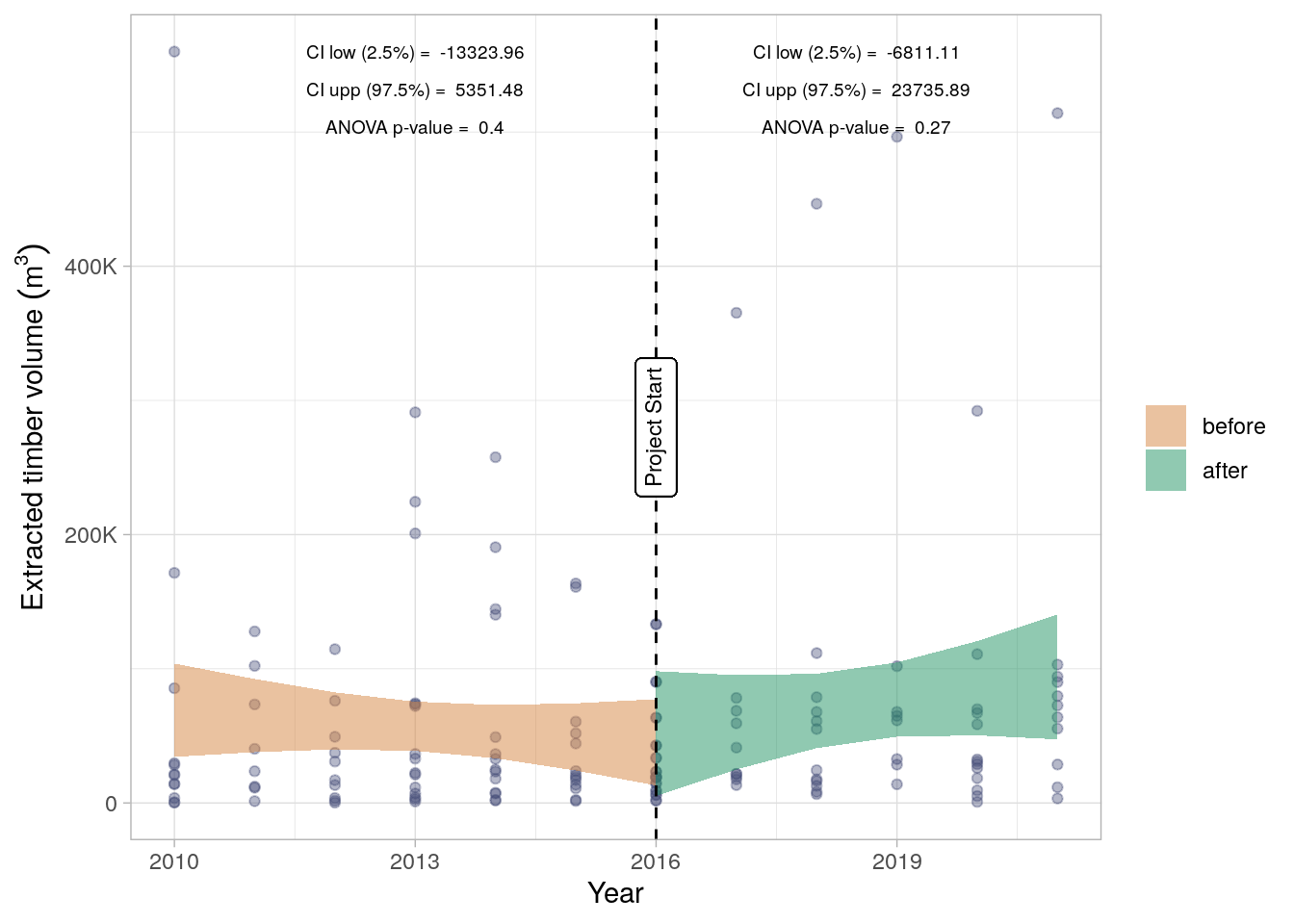
Extracted timber volumes, derived from non-plantation concessions across Sabah, were compared over time to determine if there was a statistically significant trend in timber extraction since the commencement of the Kuamut project. In line with section 8.3.1 of the VM0010 methods, fit two linear models to the data one for data from 2010 to 2016 (the project start date) and another for data from 2016 to 2021 (Figure 19.1). Neither model demonstrates a statistically significant trend with widely varying confidence intervals of the slope. The slope confidence range spans below and above zero demonstrating that there is no evidence for a trend in timber extraction either prior to or after the commencement of the Kuamut project. Any leakage as a result of the project is therefore not observable at the market-level.

Figure 19.1: Reported extracted timber volume from non-plantation concessions across Sabah between 2010 and 2021. The orange ribbon indicates the 95% confidence interval (CI) for the linear model fit for the period before project start. The green ribbon indicates the 95% CI for the linear model fit for the period after project start.

19.2 Market leakage Factor:

Whilst no change in leakage has been observed across the state of Sabah (Figure Figure 19.1), The VM0010 methodology requires the calculation of a market leakage factor according to the methods in Box 2: Leakage Factor Calculation. A summary table of these calculations and the deductions is given below in Table 19.1. These factors are applied to the final emissions reductions estimates as calculated in Chapter 21.

The quantification of the following variables is required to derive the leakage factor:

• The ratio of merchantable biomass to total biomass (PMPi) of each strata (or in our case, the management strata, i.e., Mosaic and NFM).

• The ratio of merchantable biomass to total biomass for each forest type (PMLFT); which we derived from all concessions in Sabah under the same management type.

To ensure consistent biomass predictions between the Kuamut Project and other Sabah concessions, we used biomass maps from Asner et al. (2018). We calculated PMPi by dividing the annual baseline timber harvest density, for each management stratum (see Chapter 11 and Chapter 12), by the biomass density in that stratum. For PMLFT, we divided the total reported merchantable biomass density, for each concession, by the biomass density of that concession.

The final leakage factors are derived based on the thresholds given in Box 2: Leakage Factor Calculation. An area-weighted average of the leakage factor was then calculated, in line with the VM0010 methodology, to derive the final leakage factor for the project of 0.288, which was applied in Chapter 21.

Table 19.1: A summary table displaying the market leakage values and the associated deduction factors for the different strata.

19.3 Code

#' Combine timber production files
#' timber production files are provided by the Sabah Forestry Department. This
#' function combines them into a single file for analysis.
#' @param tp10_19 file path (character) to the timber production csv for 2010
#' to 2019.
#' @param tp20_21 file path (character) to the timber production csv for 2020
#' to 2021.
#' @param outdir directory (character) to save the combined timber production
#' file.
#' @param impute_missing_areas logical, if TRUE (default) then missing harvest
#' areas are imputed using the mean harvest area to volume ratio for that
#' forest reserve and land use type.
#' @return file path (character) to the combined timber production csv.
#' @details Timber production data are provided by the Sabah Forestry
#' Department (SFD) in two separate files, one covering 2010 to 2019 and
#' another covering 2020 to 2021. This function combines these files into a
#' single dataframe for analysis.
combine_timber_production_files <- function(
  tp10_19,
  tp20_21, # TODO: generalise to ... to enable new files to be added
  outdir = "data_out/RoutputProducts/TimberProduction"
) {
  checkmate::assert_character(tp10_19)
  checkmate::assert_character(tp20_21)

  # Import timber product data from 2010 to 2020.
  timber_production_10_to_19 <- readr::read_csv(
    tp10_19,
    show_col_types = FALSE
  ) |>
    dplyr::select(-IDNo) |> # Remove ID column
    # Combine one contractor 'SAPULUT FR. (BORNION)' with the rest of that
    # reserve 'SAPULUT FR'
    dplyr::mutate(
      ForestReserve = dplyr::case_when(
        ForestReserve == "SAPULUT FR. (BORNION)" ~ "SAPULUT FR.",
        TRUE ~ ForestReserve
      )
    )

  # Import Timber Production from SFD, 2020 - 2021
  timber_production_20_to_21 <- readr::read_csv(
    tp20_21,
    show_col_types = FALSE
  ) |>
    # Remove ID column
    dplyr::select(-IDNo) |>
    # Fix the name
    dplyr::rowwise() |>
    dplyr::mutate(
      ForestReserve = find_reserve_name(
        timber_production_10_to_19$ForestReserve,
        ForestReserve
      )
    )

  # Combine Timber Production 2009 to 2019 and 2020 to 2021
  # Consideration of planted timber is inappropriate - this timber is ear-marked
  # for harvesting and is not subject to the same constraints as natural forest
  # timber.
  # Data are summarised by year, forest reserve and land use so that the
  # mean intensity of timber harvest can be assessed across all relevant
  # concession types annually.

  tpd <- dplyr::bind_rows(
    timber_production_10_to_19,
    timber_production_20_to_21
  ) |>
    dplyr::filter(LandUse != "PlantedTimber", HarvestVolume > 0) |>
    dplyr::group_by(YEAR, ForestReserve, LandUse) |>
    dplyr::summarise(
      HarvestVolume = sum(HarvestVolume),
      HarvestArea = sum(HarvestArea),

      Vol_ha = HarvestVolume / HarvestArea,
      .groups = "drop"
    )

  fs::dir_create(outdir)
  outfile <- file.path(outdir, "SabahTimberProduction_2010_2021.csv")
  readr::write_csv(
    tpd,
    outfile
  )
  return(outfile)
}


#' Find the reserve name
#' @param forest_reserve A vector of forest reserve names
#' @param pattern A string to match
#' @param max_distance Maximum distance for agrep
#' @return a string of the matched reserve names
#' @details Names of forest reserves are written differently. This function
#' uses fuzzy matching to increase distance until the first match is found.
find_reserve_name <- function(forest_reserve, pattern, max_distance = 0.1) {
  matches <- agrep(
    pattern,
    unique(forest_reserve),
    ignore.case = TRUE,
    value = TRUE,
    max.distance = max_distance,
    useBytes = TRUE
  )

  if (length(matches) == 0) {
    if (max_distance == 1.0) {
      matches <- NA
      warning(sprintf(
        "length of returned match is %s for '%s'",
        matches,
        pattern
      ))
    } else {
      new_max_distance <- max_distance + 0.1
      matches <- find_reserve_name(forest_reserve, pattern, new_max_distance)
    }
  } else if (length(matches) > 1) {
    warning(sprintf(
      "The length of the returned match is %s for '%s'",
      matches,
      pattern
    ))
  }
  return(matches)
}

#'  Activity Shifting leakage
#'
#' Function to analyse the trend in timber production from across Sabah.
#'
#' @param TP_src Timber production file 2010-2019
#' @param TPmr_src Timber production file 2020-2021
#' @param model_type Type of model to use for the analysis.
#' Default is 'segmented'.
#' @param ... Additional arguments to pass to the segmented::seg.control
#' function. only used if model_type = 'segmented'.
#'
#' @return a list of outputs including combined tables, plots and linear models.
estimate_act_shift_leakage <- function(
  tp,
  proj_start = 2016,
  tab_path = "data_out/Routputs/Tables"
) {
  # --------------------------- input assertion ---------------------------#
  checkmate::assert_character(tp)
  checkmate::assert_numeric(proj_start)

  # --------------------------- data pre processing ---------------------------#

  tpd <- readr::read_csv(tp)

  split_mod_df <- join_before_after_fits(tpd, proj_start)

  timb_prod_plot <- save_timber_production_plot(split_mod_df, proj_start)

  # Write the full dataset on activity leakage (acl)
  tpd |>
    rename_all(
      ~ c(
        "Year",
        "Forest Reserve",
        "Logging Type",
        "Harvest Volume (m3)",
        "Harvest Area (ha)",
        "Volume per hectare (m3 ha-1)"
      )
    ) |>
    export_tab_n_csv(
      "ActivityLeakageYearTable",
      tab_path
    )

  return(list(
    TimbProd_plot = timb_prod_plot$plot,
    TimbProd_plot_path = timb_prod_plot$path
  ))
}

#' Linear model predictions for leakge analysis
#' @param df Dataframe to predict
#' @param .period Period of the prediction a character: "before" or "after
#' @return a dataframe with the predictions and the model object as an attribute
#'
linear_preds <- function(df, .period = c("before", "after")) {
  .period <- rlang::arg_match(.period)

  timber_prod_mod <- lm(HarvestVolume ~ YEAR, data = df)

  df <- dplyr::bind_cols(
    df,
    predict(
      timber_prod_mod,
      newdata = df,
      interval = "confidence",
      level = 0.95,
      type = "response"
    )
  ) |>
    mutate(period = .period)

  model_cis <- confint(timber_prod_mod)
  ci_025 <- round(model_cis[2], 3)
  ci_975 <- round(model_cis[4], 3)

  aov_p_value <- round(anova(timber_prod_mod)$`Pr(>F)`[1], 3)

  mod_attrs <- list(timber_prod_mod, ci_025, ci_975, aov_p_value)

  return(list(
    data = df,
    model_attrs = mod_attrs
  ))
}


#' Create and save a timber production plot
#' @param data Dataframe to plot containing before and after model attributes
#' @param proj_start Project start year
#' @param filename Name of the file to save the plot
#' @param out_dir Directory to save the plot
#' @return a list containing the plot and the path to the saved plot
save_timber_production_plot <- function(
  data,
  proj_start,
  filename = "ActivityShiftingLeakageGraph_MR.png",
  out_dir = "data_out/Routputs"
) {
  # set up labelling locations
  leak_start <- min(data$YEAR)
  leak_end <- max(data$YEAR)
  before_cent <- leak_start + (proj_start - leak_start) / 2
  after_cent <- proj_start + (leak_end - proj_start) / 2
  lab_upper <- max(data$HarvestVolume)

  # custom annotation function
  an_add <- function(x, y, z, c = before_cent) {
    ggplot2::annotate(
      "text",
      x = c,
      y = lab_upper * z,
      size = 2.5,
      label = paste(x, y)
    )
  }

  # Plot the timber production
  timber_plot <- data |>
    ggplot() +
    aes(x = YEAR, y = HarvestVolume) +
    geom_point(alpha = 0.4, colour = "#484f79") +
    geom_ribbon(
      data = data,
      aes(ymin = lwr, ymax = upr, fill = period),
      alpha = 0.5
    ) +
    geom_vline(xintercept = proj_start, linetype = "dashed") +
    labs(
      x = "Year",
      y = bquote("Extracted timber volume" ~ (m^3)),
      fill = ""
    ) +
    scale_fill_manual(values = c("#d68543", "#239465")) +
    # scale_y_log10() +
    theme_light() +
    an_add("CI low (2.5%) = ", attributes(data)$before_ci_025, 1) +
    an_add("CI upp (97.5%) = ", attributes(data)$before_ci_975, 0.95) +
    an_add("ANOVA p-value = ", attributes(data)$before_aov_p_value, 0.9) +
    an_add(
      "CI low (2.5%) = ",
      attributes(data)$after_ci_025,
      1,
      after_cent
    ) +
    an_add(
      "CI upp (97.5%) = ",
      attributes(data)$after_ci_975,
      0.95,
      after_cent
    ) +
    an_add(
      "ANOVA p-value = ",
      attributes(data)$after_aov_p_value,
      0.9,
      after_cent
    ) +
    ggtext::geom_richtext(
      aes(
        x = proj_start,
        y = lab_upper / 2,
        label = "Project Start"
      ),
      size = 3,
      angle = 90,
      fill = "white"
    ) +
    scale_y_continuous(
      labels = scales::label_number(scale_cut = scales::cut_short_scale())
    )

  # Save plot to system
  timber_plot_path <- set_path(filename, out_dir)
  ggsave(filename = timber_plot_path, plot = timber_plot)

  # Return both the plot and the path
  return(list(
    plot = timber_plot,
    path = timber_plot_path
  ))
}


#' wrapper to create the timber production models pre post project.
#' @param tpd_data Timber production dataframe
#' @param proj_start Project start year
#' @return a dataframe with the predictions and the model objects, their
#' confidence intervals and ANOVA p-values as attributes.
#' @details The function splits the data into two periods, before and after
#' the project start year. It then fits a linear model to each period and
#' returns a dataframe with the predictions and the model objects, their
#' confidence intervals and ANOVA p-values as attributes.
join_before_after_fits <- function(tpd_data, proj_start) {
  tpd_pre_prj <- tpd_data |>
    dplyr::filter(YEAR <= proj_start) |>
    linear_preds("before")

  tpd_post_prj <- tpd_data |>
    dplyr::filter(YEAR >= proj_start) |>
    linear_preds("after")

  split_mod_df <- bind_rows(
    tpd_pre_prj$data,
    tpd_post_prj$data
  ) |>
    dplyr::mutate(period = factor(period, levels = c("before", "after"))) |>
    add_attrs(tpd_pre_prj$model_attrs, "before") |>
    add_attrs(tpd_post_prj$model_attrs, "after")

  return(split_mod_df)
}

#' Add attributes to a dataframe
#' @param x Dataframe to add attributes to
#' @param y List of attributes to add
#' @param .period Period of the prediction a character: "before" or "after"
#' @param pr Number of decimal places to round to
#' @return a dataframe with the attributes added
#' @details The function adds the model, confidence intervals and ANOVA p-values
#' to the dataframe.
add_attrs <- function(x, y, .period = c("before", "after"), pr = 2) {
  .period <- rlang::arg_match(.period)
  attr(x, paste0(.period, "_model")) <- y[[1]]
  attr(x, paste0(.period, "_ci_025")) <- round(y[[2]], pr)
  attr(x, paste0(.period, "_ci_975")) <- round(y[[3]], pr)
  attr(x, paste0(.period, "_aov_p_value")) <- round(y[[4]], pr)
  return(x)
}

#' Leakage Estimation
#'
#' This function estimates the leakage factor for the project area based on the
#' ratio of merchantable biomass to total biomass across all strata in the base
#' year, and the ratio of merchantable biomass to total biomass of the country's
#' forest estate where harvesting would likely be displaced to.
#'
#' @param TP_src Timber Production source file.
#' @param FRs_src Forest Reserves source file - a geospatial polygon of forest
#' reserves.
#' @param FRnames_src Forest Reserve names source file.
#' @param CAO_Sabah_src CAO carbon map source file. Covering the whole of Sabah.
#' from Asner, et. al. (2018).
#' @param Boundary_src Project boundary source file. Spatial polygon
#' @param Mosaic_src Mosaic strata source file. Spatial polygon
#' @param NFMCoupes_src NFM strata source file. Spatial polygon
#' @param Mosaic_Parcels_csv Mosaic parcels baseline timber harvest predictions
#' from `R/TimberHarvestPlan_Mosaic_Coupes.R`.
#' @param NFM_Parcels_csv NFM parcels baseline timber harvest predictions from
#' `R/TimberHarvestPlan_NFM_Coupes.R`.
#' @param BCEF_R Biomass Conversion and Expansion Factor for Sabah.
#' @param CF Carbon Fraction.
#'
#' @return A list of outputs including: leakge factors for NFM and Mosiac
#' strata, forest reserve outlines, CSV files, and tables.
#' @details   # VM0010v1.3 (page 49)
#' basis of a comparison between the ratio of merchantable biomass to total
#' biomass across all strata in the base year, and the ratio of merchantable
#' biomass to total biomass of the country's forest estate where
#' harvesting would likely be displaced to.
#' we therefore only use the data including and after 2016 (== base year, and
#' corresponding displacement years)
estimate_market_leakage <- function(
  tp,
  FRs_src,
  FRnames_src,
  CAO_Sabah_src,
  Boundary_src,
  Mosaic_src,
  NFMCoupes_src,
  Mosaic_Parcels_csv,
  NFM_Parcels_csv,
  BCEF_R = 1.89,
  CF = 0.47
) {
  TP <- readr::read_csv(tp) |>
    dplyr::filter(
      YEAR >= 2016,
      LandUse != "PlantedTimber",
      # Some areas reported without extraction, so remove NA's and zeroes
      !is.na(HarvestVolume),
      HarvestVolume > 0
    )

  ActLeakFRs <- TP |>
    dplyr::group_by(ForestReserve, LandUse) |>
    dplyr::summarise(
      HarvestArea = sum(HarvestArea, na.rm = TRUE),
      HarvestVolume = sum(HarvestVolume, na.rm = TRUE)
    )

  ActLeakForestResTab.doc <- export_ActLeakFRs(ActLeakFRs)

  # Names of Forest Reserves as per CAO carbon map
  FRnames <- read.csv(FRnames_src)

  # CAO carbon map 2016 in base year
  CAO_Sabah <- terra::rast(CAO_Sabah_src)

  ## All Sabah ForestReserves carbon explore
  FR_outlines <- sf::read_sf(FRs_src)

  FR_outlines <- dplyr::rename(FR_outlines, ForestReserve = FOREST_NA)

  # Subset the Forest reserve outlines that have active logging during
  # reporting period
  FR_outlines <- FR_outlines |>
    dplyr::filter(ForestReserve %in% c(TP$ForestReserve))

  # save file for map for PD
  fr_base <- set_path("RoutputProducts/ActiveFReserveOutlines")
  fs::dir_create(fr_base)
  FR_outlines_shp <- file.path(fr_base, "ActiveFReserveOutlines.shp")

  suppressWarnings(
    # supress warings becuase shp files are silly.
    sf::write_sf(
      FR_outlines,
      FR_outlines_shp,
      delete_dsn = TRUE,
      append = FALSE
    )
  )

  ## CORRECT UNITS
  # we want to sum them up, so values need to be per pixel
  scale_fac <- function(x) {
    rasres <- terra::res(x)
    (rasres[1] * rasres[2]) / (100 * 100)
  }

  # scale by 0.09 to give total per pixel
  CAO_Sabahperpixel <- CAO_Sabah * scale_fac(CAO_Sabah)

  dat <- FR_outlines |>
    mutate(
      ACDsum = round(
        exactextractr::exact_extract(CAO_Sabahperpixel, FR_outlines, "sum"),
        1
      ),
      FR_Area = round(
        as.numeric(units::set_units(sf::st_area(FR_outlines), ha)),
        1
      )
    )

  # We have extracted the ACD and summed it per forest reserve
  # but each reserve may have multiple polygons
  # so we now aggregate to one value per Forest reserve

  # aggregate with dplyr
  datGr <- dat |>
    dplyr::group_by(ForestReserve) |>
    dplyr::summarise(
      TotC = sum(ACDsum, na.rm = TRUE),
      FR_Area = sum(FR_Area, na.rm = TRUE)
    ) |>
    mutate(
      # calculate average ACD (i.e per hectare not sum) per Forest Reserve
      ACD = round(TotC / FR_Area, 1),
      ## convert Carbon to Biomass using Carbon Fraction
      AGB = ACD / CF
    ) |>
    dplyr::select(ForestReserve, AGB)

  # summarise extraction data by forest reserve and
  # forest type (NFM of Salvage logging)

  # calculate merchantable biomass from merchantable volume using BCEF_R
  # Average Timber Production grouped by ForestReserve and LandUse
  # We average at this resolution (FR), because this is the same resolution that is possible for the biomass
  # i.e we cannot get shapefiles at a higher resolution than forest reserves.
  # the aggregation at FR level is therefor comparable.
  AllDat <- TP |>
    group_by(ForestReserve, LandUse) |>
    dplyr::summarise(Vol_ha = mean(Vol_ha, na.rm = TRUE), .groups = "drop") |>
    mutate(MerchBiomass = Vol_ha * BCEF_R) |>
    select(ForestReserve, LandUse, MerchBiomass) |>
    ## merge biomass map data with extracted volume data
    right_join(sf::st_drop_geometry(datGr), by = "ForestReserve") |>
    ## The salvage logging in BENGKOKA FR left 0 AGB behind,
    # replace with lowest denisty measured elsewhere
    dplyr::mutate(
      AGB = dplyr::case_when(
        AGB == 0 ~ min(datGr$AGB[datGr$AGB > 0]),
        TRUE ~ AGB
      )
    ) |>
    # ratio of merchantable biomass to total biomass (PMPi)
    # PML Ratio of merchantable biomass to total biomass
    # VM0010v1.4 (pages 49-50)
    mutate(PML = MerchBiomass / AGB) |>
    relocate(AGB, .before = LandUse)

  all_dat_exports <- export_AllDat(AllDat)

  # Follow Exactly the same method for our project area
  # USE CAO carbon map so corresponds directly
  # Project Boundary
  Boundary <- sf::read_sf(Boundary_src)

  # For our project area we can separately extract ACD for each strata -
  # NFM and Mosaic, more accurate for each Area for Mosaic Plantings
  read_strata <- function(src, .id) {
    sf::read_sf(src) |>
      dplyr::summarise() |>
      mutate(Strata = .id)
  }

  Project <- read_strata(Mosaic_src, "Mosaic") |>
    bind_rows(read_strata(NFMCoupes_src, "NFM"))

  Project <- Project |>
    mutate(
      Area = as.numeric(units::set_units(sf::st_area(Project), "ha")),
      TotC = exactextractr::exact_extract(CAO_Sabahperpixel, Project, "sum"),
      ACD = TotC / Area,
      AGB = ACD / CF
    )

  # Use  V_EX directly from Timber Harvest plan (Parcels)
  Mosaic_Parcels <- read.table(Mosaic_Parcels_csv) |>
    ## just the first round of logging makes sense
    dplyr::filter(Rotation == "First")

  # we have the two mosaic strata separated, which doesn't compare to the data
  # for the rest of the state- so we combine here with weighted average
  Mosaic_Parcels2 <- Mosaic_Parcels |>
    dplyr::rename(Area_coupe = Area_ha) |>
    group_by(LogYear) |>
    dplyr::summarise(
      VolSum = sum(VolSum, na.rm = TRUE),
      Area_ha = sum(Area_coupe, na.rm = TRUE),
      # the correct way to average. as this corresponds to what is propagated
      V_EX = weighted.mean(V_EX, w = Area_coupe),
      Strata = "Mosaic",
      Plant = "planted",
      Rotation = "First"
    )

  NFM_Parcels <- read.table(NFM_Parcels_csv) |>
    dplyr::filter(Rotation == "First")

  # join parcel dfs.
  Parcels <- rbind(Mosaic_Parcels2, NFM_Parcels) |>
    # calculate merchantable biomass from merchantable volume using BCEF_R
    mutate(MerchBiomass = V_EX * BCEF_R) |>
    left_join(sf::st_drop_geometry(Project), by = "Strata") |>
    mutate(PMP_I = MerchBiomass / AGB)

  PrjLeak <- Parcels |>
    group_by(Strata) |>
    dplyr::summarise(
      PMP_I = mean(PMP_I, na.rm = TRUE),
      MerchBiomass = mean(MerchBiomass, na.rm = TRUE),
      AGB = mean(AGB, na.rm = TRUE),
      Area_ha = sum(Area_ha, na.rm = TRUE)
    )

  pmpexp <- prj_leak_export(PrjLeak)

  ### For the FR's in the Rest of Sabah PML - FT

  # relevel first makes the table order match later
  AllDat$LandUse <- factor(AllDat$LandUse, levels = c("SalvageLogging", "NFM"))

  Dat_FT <- AllDat |>
    group_by(LandUse) |>
    dplyr::summarise(
      PML_FT = mean(PML, na.rm = TRUE),
      MerchBiomass = mean(MerchBiomass, na.rm = TRUE),
      AGB = mean(AGB, na.rm = TRUE)
    )

  # In both strata the baseline extracts less than the rest of the state does

  # write table for PD done above
  # Save table in word doc format
  dat_ft_exp <- export_dat_ft(Dat_FT)

  #----------------------------------------------------------------------------#
  # -------------- Leakage factor calculation  --------------------------------#
  #----------------------------------------------------------------------------#

  # function based on leakage thresholds described on p. 50 of the VM0010,
  # Version 1.3 methodology

  # Define PML_FT and PMP_I for NFM
  PML_FT_NFM <- subset(Dat_FT, LandUse == "NFM")$PML_FT
  PMP_I_NFM_PRJ <- subset(PrjLeak, Strata == "NFM")$PMP_I

  # In the NFM the Ratio is Higher in the project area
  cli::cli_alert_info("NFM Leakage:")

  nfm_leak_sum <- leakage_factor(PML_FT_NFM, PMP_I_NFM_PRJ)
  NFM_LFME <- nfm_leak_sum$lfme

  # Define PML_FT and PMP_I for Mosaics
  PML_FT_Mos <- subset(Dat_FT, LandUse == "SalvageLogging")$PML_FT

  PMP_I_MosPRJ <- subset(PrjLeak, Strata == "Mosaic")$PMP_I
  # In the Mosaic the Ratio is LOWER in the project area
  cli::cli_alert_info("Mosaic Leakage:")
  mosaic_leak_sum <- leakage_factor(PML_FT_Mos, PMP_I_MosPRJ)
  MOSAIC_LFME <- mosaic_leak_sum$lfme

  leakage_summary <- export_leakage_summary(
    PMP_I_NFM_PRJ,
    PMP_I_MosPRJ,
    PML_FT_NFM,
    PML_FT_Mos,
    nfm_leak_sum,
    mosaic_leak_sum,
    NFM_LFME,
    MOSAIC_LFME
  )

  return(
    list(
      nfm_LFME = NFM_LFME,
      mosaic_LFME = MOSAIC_LFME,
      forest_reserve_outlines = FR_outlines_shp,
      PML_FT_csv = dat_ft_exp$PML_FT.csv,
      PMP_I_csv = pmpexp$PMP_I.csv,
      leak_sum = leakage_summary$leak_sum,
      table_exports = list(
        ActLeakForestResTab.doc,
        all_dat_exports$PML_FTtab.doc, #check
        all_dat_exports$PML_ActiveLoggingCoupes.csv,
        all_dat_exports$PML_ActiveLoggingCoupes.doc,
        pmpexp$PMP_I_ProjectArea.doc,
        dat_ft_exp$PML_FT.doc,
        leakage_summary$leak_sum.doc
      )
    )
  )
}


export_ActLeakFRs <- function(ActLeakFRs) {
  ActLeakForestResTab.doc <- set_path(
    "Routputs/Tables/ActivityLeakageForestReservesTable.docx"
  )

  ActLeakFRs |>
    rename_all(
      ~ c(
        "Forest Reserve",
        "Logging Type",
        "Harvest Area (ha)",
        "Harvest Volume (m3)"
      )
    ) |>
    gt_tab(
      .filename = ActLeakForestResTab.doc,
      .digits = 1
    )

  return(ActLeakForestResTab.doc)
}


export_AllDat <- function(AllDat) {
  ## Save PML (for each FR) table for PD in word doc format
  PML_FTtab.doc <- set_path("Routputs/Tables/PML_FTtab.docx")

  AllDat |>
    rename_all(
      ~ c(
        "Forest Reserve",
        "AGB (mg/ha)",
        "Logging Type",
        "Merchantable Biomass",
        "PML"
      )
    ) |>
    gt_tab(
      .filename = PML_FTtab.doc,
      .digits = 4
    )

  ## save CSV table for Marco / PD
  PML_ActiveLoggingCoupes.csv <- set_path(
    "Routputs/Tables/PML_ActiveLoggingCoupes.csv"
  )
  write.csv(AllDat, PML_ActiveLoggingCoupes.csv, row.names = FALSE)

  # Save table in word doc format (for consistency, not an essential output)
  PML_ActiveLoggingCoupes.doc <- set_path(
    "Routputs/Tables/PML_ActiveLoggingCoupes.docx"
  )

  gt_tab(AllDat, .filename = PML_ActiveLoggingCoupes.doc, .digits = 5)

  list(
    PML_ActiveLoggingCoupes.csv = PML_ActiveLoggingCoupes.csv,
    PML_ActiveLoggingCoupes.doc = PML_ActiveLoggingCoupes.doc,
    PML_FTtab.doc = PML_FTtab.doc
  )
}


prj_leak_export <- function(PrjLeak) {
  PMP_I_ProjectArea.doc <- set_path("Routputs/Tables/PMP_I_ProjectArea.docx")

  PrjLeak |>
    rename_all(
      ~ c(
        "Stratum",
        "PMP_I",
        "Merchantable Biomass",
        "AGB (mg/ha)",
        "Area (ha)"
      )
    ) |>
    gt_tab(
      .filename = PMP_I_ProjectArea.doc,
      .digits = 4
    )

  PMP_I.csv <- set_path("Routputs/PMP_I.csv")
  write.csv(PrjLeak, PMP_I.csv)

  return(list(
    PMP_I_ProjectArea.doc = PMP_I_ProjectArea.doc,
    PMP_I.csv = PMP_I.csv
  ))
}


export_dat_ft <- function(Dat_FT) {
  PML_FT.doc <- set_path("Routputs/Tables/PML_FT.docx")
  Dat_FT |>
    dplyr::select(LandUse, PML_FT, MerchBiomass, AGB, PML_FT) |>
    rename_all(
      ~ c(
        "Logging Type",
        "PMP_FT",
        "Merchantable Biomass",
        "AGB (mg/ha)"
      )
    ) |>
    gt_tab(
      .filename = PML_FT.doc,
      .digits = 5
    )

  # Dat_FT = data.frame(Dat_FT[,1], round(Dat_FT[,-1], 3))
  PML_FT.csv <- set_path("Routputs/PML_FT.csv")
  Dat_FT |>
    select(LandUse, PML_FT, MerchBiomass, AGB, PML_FT) |>
    write.csv(PML_FT.csv)

  list(
    PML_FT.csv = PML_FT.csv,
    PML_FT.doc = PML_FT.doc
  )
}

#' Calculate the leakage factor according to the VM0010v1.4 guidelines
#' @param pml_ft Ratio of merchantable biomass to total biomass in the
#' corresponding forest type in the rest of Sabah (PML FT)
#' @param pmp_i Ratio of merchantable biomass to total biomass in the project
#' area (PMP i)
#' @return A list with the leakage factor (lfme) and the percentage difference
#' between PML FT and PMP i (perc_diff)
#' @details
#' If PML FT is within 15% of PMP i, LFME = 0.4
#' If PML FT is more than 15% lower than PMP i, LFME = 0.7
#' If PML FT is more than 15% higher than PMP i, LFME = 0.2
#' @seealso
#' https://verra.org/wp-content/uploads/2024/10/VM0010_IFM_LtPF_v1.4_Clean_10282024.pdf#page=48
leakage_factor <- function(pml_ft, pmp_i) {
  inc <- pml_ft - pmp_i
  perc_diff <- round((inc / pmp_i) * 100, 2)
  if (perc_diff > 0) {
    direction <- "more"
  } else {
    direction <- "less"
  }
  message(paste0(
    "PML FT is ",
    abs(perc_diff),
    "% ",
    direction,
    " than PMP i"
  ))

  if (perc_diff < 15 && perc_diff > -15) {
    lfme <- 0.4
  } else if (perc_diff < -15) {
    lfme <- 0.7
    warning(sprintf("LEAKAGE FACTOR CALCULATED AS %s!!!", lfme))
  } else if (perc_diff > 15) {
    lfme <- 0.2
  }
  message(sprintf("Leakage Factor is %s", lfme))
  return(list(
    lfme = lfme,
    perc_diff = perc_diff
  ))
}


export_leakage_summary <- function(
  PMP_I_NFM_PRJ,
  PMP_I_MosPRJ,
  PML_FT_NFM,
  PML_FT_Mos,
  nfm_leak_sum,
  mosaic_leak_sum,
  NFM_LFME,
  MOSAIC_LFME
) {
  leak_sum <- tibble(
    `Stratum in project area` = c("Stratum 2", "Stratum 3 and 4"),
    `Corresponding forest type` = c(
      "Natural Forest Management",
      "Salvage Logging"
    ),
    `PMPi` = round(c(PMP_I_NFM_PRJ, PMP_I_MosPRJ), 2),
    `PMLft` = round(c(PML_FT_NFM, PML_FT_Mos), 2),
    `% difference between PMPi and PMLft` = c(
      nfm_leak_sum$perc_diff,
      mosaic_leak_sum$perc_diff
    ),
    `Deduction Factor (LF_ME)` = c(NFM_LFME, MOSAIC_LFME)
  )

  leak_sum.doc <- set_path("Routputs/Tables/leak_sum.docx")

  gt_tab(leak_sum, .filename = leak_sum.doc, .digits = 5)
  return(list(
    leak_sum = leak_sum,
    leak_sum.doc = leak_sum.doc
  ))
}

Asner, Gregory P, Philip G Brodrick, Christopher Philipson, Nicolas R Vaughn, Roberta E Martin, David E Knapp, Joseph Heckler, et al. 2018. “Mapped Aboveground Carbon Stocks to Advance Forest Conservation and Recovery in Malaysian Borneo.” Biological Conservation 217: 289–310.