7 Biomass Mapping
In order to quantify the biomass growth rates and the total emissions lost due to degradation, we have developed a multi-temporal modelling approach to estimate the spatial variability and distribution of aboveground biomass.
To achieve this we have adopted a machine learning workflow that uses the following data sources: aerial LiDAR scan (ALS) data from 2016 describing canopy height, USGS Landsat 8 Level 2, Collection 2, Tier 1, Sentinel-1 SAR GRD: C-band Synthetic Aperture Radar Ground Range Detected, log scaling, and forest plot data from the Kuamut Project area.
These data are used as inputs to a Machine Learning Pipeline, the structure of which is depicted in Figure 7.1 below:
7.1 Input data Aquisition and Processing.
7.1.1 Landsat 8
Annual composites of Landsat 8 (L8) imagery were created for the Kuamut project area using Google earth engine. All images, in a given year, with a cloud cover faction < 50% were retained, cloud masking of images was carried out using the rgeeExtra package (Aybar et al. 2020). L8 values were then rescaled to provide the correct floating point value for each band. The following spectral indices (presented in Table 7.1) were then calculated using {rgeeExtra} package (Aybar et al. 2020)- see Awesome Spectral Indices (David Montero 2022) for further information:
Median composite L8 images were then generated for years 2015:2022. The following bands were removed from the resulting rasters as they were not considered to be informative for the purposes of biomass estimation and/or contained significant data gaps: Aerosol Quality Assessment, Emissivity standard deviation, Pixel Quality, Radiometric saturation, Distance to cloud, Surface temperature uncertainty.
7.1.2 Sentinel 1 (S1)
All S1 images, for a given year, that intersected the area of interest were collected. Each image was preprocessed using the following steps according to (Mullissa et al. 2021):
Erroneous values can occur on the edges of S1 imagery, these effects were masked for every image used in each annual collection.
A monotemporal Gamma despeckle filter, with a kernel size of 9 was used to reduce speckle noise in each of the images.
slope correction was then applied using a volumetric method with slope derived from SRTM 30 m data.
The Ratio between VV and VH polorizaion bands was calculated by dividing the VV band by the VH band and was subsequently converted to dB.
Each image therefore included 3 bands: VV, VH and VV:VH ratio. The median composite of all images from each year was then derived. All S1 preprocessing was carried out using Google Earth Engine and the {rgee} package (Aybar et al. 2020).
7.1.3 Terrain Data
The Copernics GLO 30 m global digital evelation model (DEM) was used to derive terrain data for the area of interest.
Further terrain metrics were derived from this DEM which included: slope, aspect, minimal curvature, mean curvature. Slope and aspect were calculated using the {terra} R package (Hijmans 2023). minimal curvature and mean curvature were calculated using the {Whitebox} R package. curvature metrics were calculated on a resampled DEM with a resoution of 150 m.
7.1.4 Temporal smoothing
Temporal smoothing/harmonisation was essential in order to enable the application of the same model across different time steps, ensuring consistent prediction and error estimates through time.
7.1.4.1 Monitoring Report 1 (2016:2021):
All the bands from the rasters discussed above were combined into a data cube, comprising a total of 41 bands. In order to harmonize the data between annual composites, it was necessary to apply temporal smoothing across each band of the data cube for all years (2015:2022). Although this Monitoring report focuses on the years 2016:2021, including years 2015 and 2022 improves the temporal smoothing estimation for those non-endpoint years and enables growth rate estimates for 2021.
This was achieved by fitting a loess regression for every cell of the data cube across time. This was applied to every band in the data cube using a span value of 2.0.
7.1.4.2 Monitoring Report 2 (2022:2023)
For this monitoring period, a full year of imagery was not yet available (2024). Therefore in order to mitigate the risk of over-fitting during the temporal smoothing process, we opted to use a linear interpolation method to smooth the data cube. The linear fit was applied for all years from 2015-2023 but only the year 2023 was carried forward for further analysis. For the MR1 period we had limited concern of over-fitting because forest plot data were collected in 2022, ensuring the constraint of predicted values for 2022. Adopting linear smoothing for 2023 conservatively allows for extrapolation in the absence of additional field data.
7.2 Canopy Height Model prediction.
A tree Canopy Height Model (CHM) was generated from LiDAR data, collected in 2016 as part of Asner et al. (2018). Using the gdalwarp utility (via the {ezwarp} package (Graham 2024)), we resampled the 2 m canopy height model to align with our data cube at a resolution of 30 m, using bilinear interpolation.
The coverage of the CHM is not complete, approximating 59260/84800 ha (~70%) of the Kuamut project area. All regions that intersected the CHM were used to create a data frame comprising the measured canopy height values from the CHM and all of the environmental/ earth observation data contained within the data cube.
7.3 Canopy Height Model Machine learning.
The {mlr3} (Lang et al. 2019) package and its ecosystem was used to structure and execute all parts of the machine learning pipeline. Spatial resampling was carried out using the {mlr3spatiotempcv} package (Schratz and Becker 2022).
Environmental variables were filtered based on the importance value, using an untrained LightGBM (LGBM) model. Then, sequential forward feature selection was used to determine the combination of environmental metrics that could produce a model with the lowest RMSE value. This was done using the default LGBM. The following features were therefore retained and used to tune and train the canopy height model: aspect, l8_CVI, l8_EVI, l8_EVI2, l8_MNLI, l8_NDVI, l8_RDVI, l8_SR_B3, l8_SR_B5, l8_SR_B6, l8_SR_B7, l8_ST_DRAD, l8_ST_URAD, l8_kVARI, s1_Ratio_RTC, s1_VH_RTC, slope.
A LGBM model was tuned, using the retained features. Spatial coordinate-based k-means clustering was used to generate resampling sets, reducing the effect of spatial autocorrelation in the selection of hypertuned parameters; 6 folds were used in each resampling iteration. Hyperband tuning was used to derive the optimal tuning parameters for the model. The following parameters were explored in the hyperparamter search space: learning_rate, max_bin, num_iterations, num_leaves. tuning parameter selection was based on a multi metric criterion, considering, the iteration RMSE and R^2.
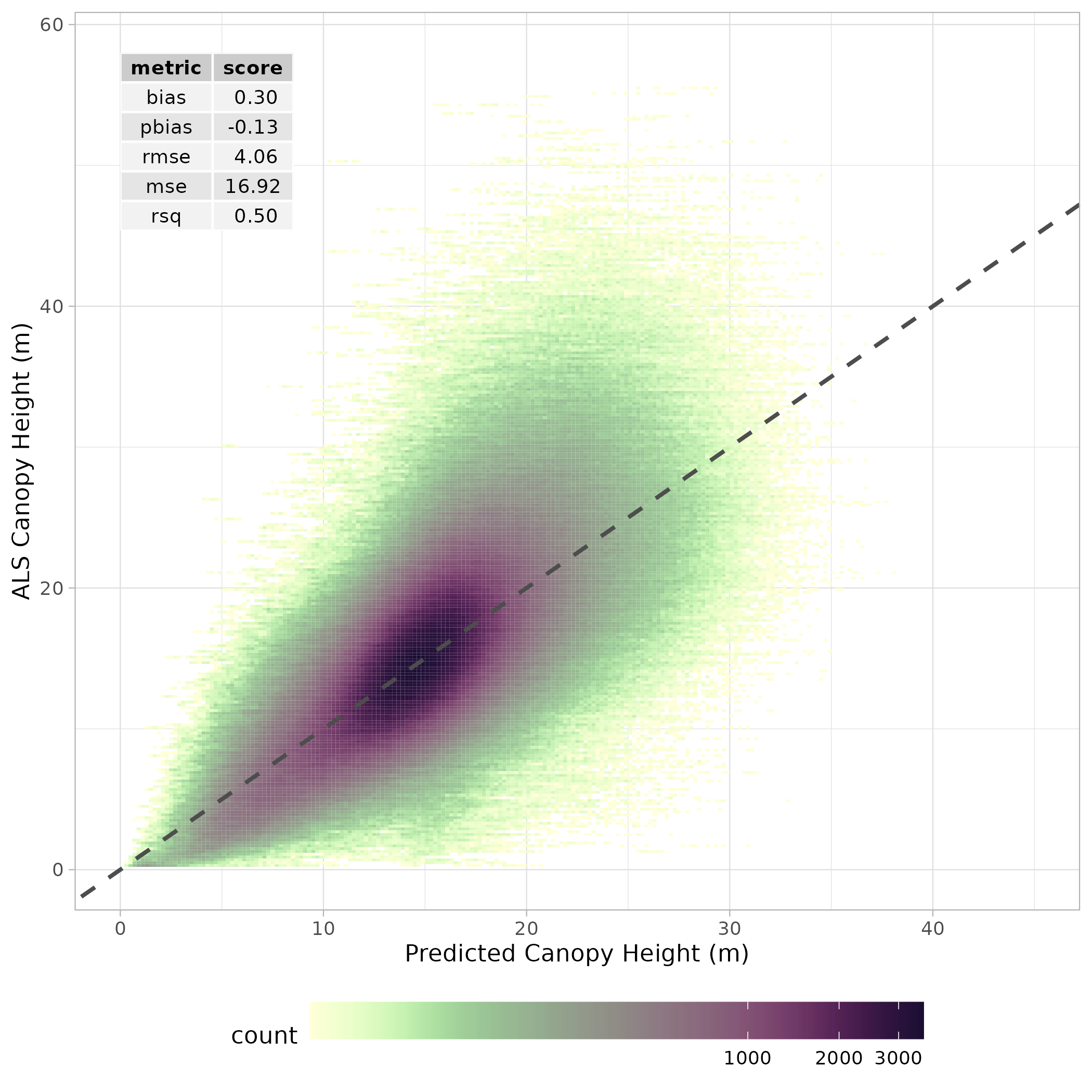
Spatial resampling was undertaken to evaluate the performance of the ensemble model. Again, a 6-fold k-means coordinate clustering approach was used to split training and test sets. The results of this cross-validation are presented in Figure 7.2.
The model was then used to predict canopy height for years 2015:2022. The resulting predictions stored as spatial raster data.
7.4 Above Ground Biomass Machine Learning model.
Canopy height model predictions for all years were appended to their respective year’s data cube as an additional band to form the input data cube for biomass model development.
Forest plots were undertaken in 2016 and 2020 in the Kuamut project area . Data cubes for the corresponding years were used to extract the environmental features that interacted each plot area for each year it was surveyed using the {exactextractr} R package, which uses a weighted calculation for partially intersected cells, providing better accuracy than an all-touches or all-contained method. The total Above Ground Carbon (AGC) was converted to Aboveground Carbon density (ACD) by dividing the AGC by the planimetric area of the plot. The derived dataframe was used to train a model to predict ACD as follows:
Manual inspection of data correlation and model performance was carried out, highlighting the following variables as being of particular importance for the prediction of ACD: Modelled canopy Height (CHM), landsat bands B1 and B7, the following spectral vegetation indices: AVI, CVI, EVIGEMI, MNLI, sentinel1 VV and VH bands, and topographic mean curvature.
The best performing model was selected using the {MuMin} R package. Here, a master model is provided containing the maximal model with all components. This included all control variables as additive effects and also the interaction between the CHM and all landsat 8 derived bands and spectral indices. All variable combinations were tested that included between 6-10 control features, two of which were required to be modelled canopy height and mean curvature (because of their importance). mean curvature identifies upland areas and ridgelines, which in the Kuamut project area are typically less effected by historical logging activity, due to their inaccessibility.
An ensemble model was then constructed from: a XGboost model from the {XGboost} R package, a support vector machine SVM, and a General Linear Model (GLM) with a gaussian family and identity link function. The predictions of these models were then combined using a ‘super learner’, in this case a simple linear regression, in line with the methods described by Polley and Van der Laan (2010). The ensemble model was constructed using the {mlr3pipelines} package Binder et al. (2021) to create a single learner which enables simultaneous tuning of all individual models.
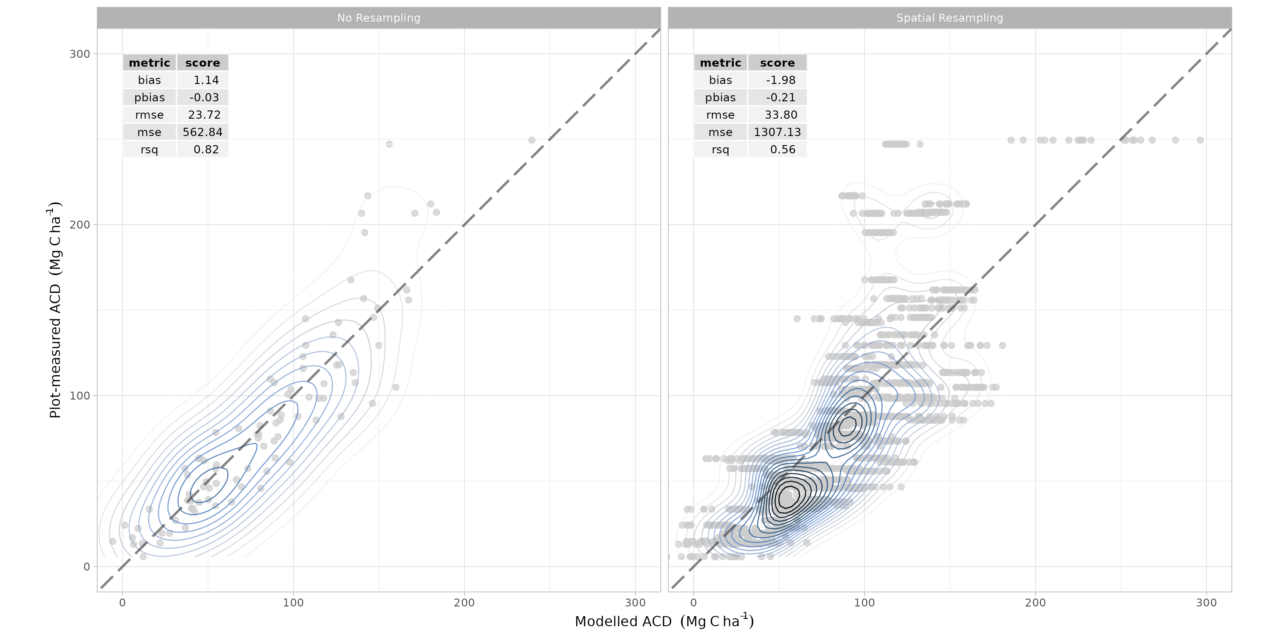
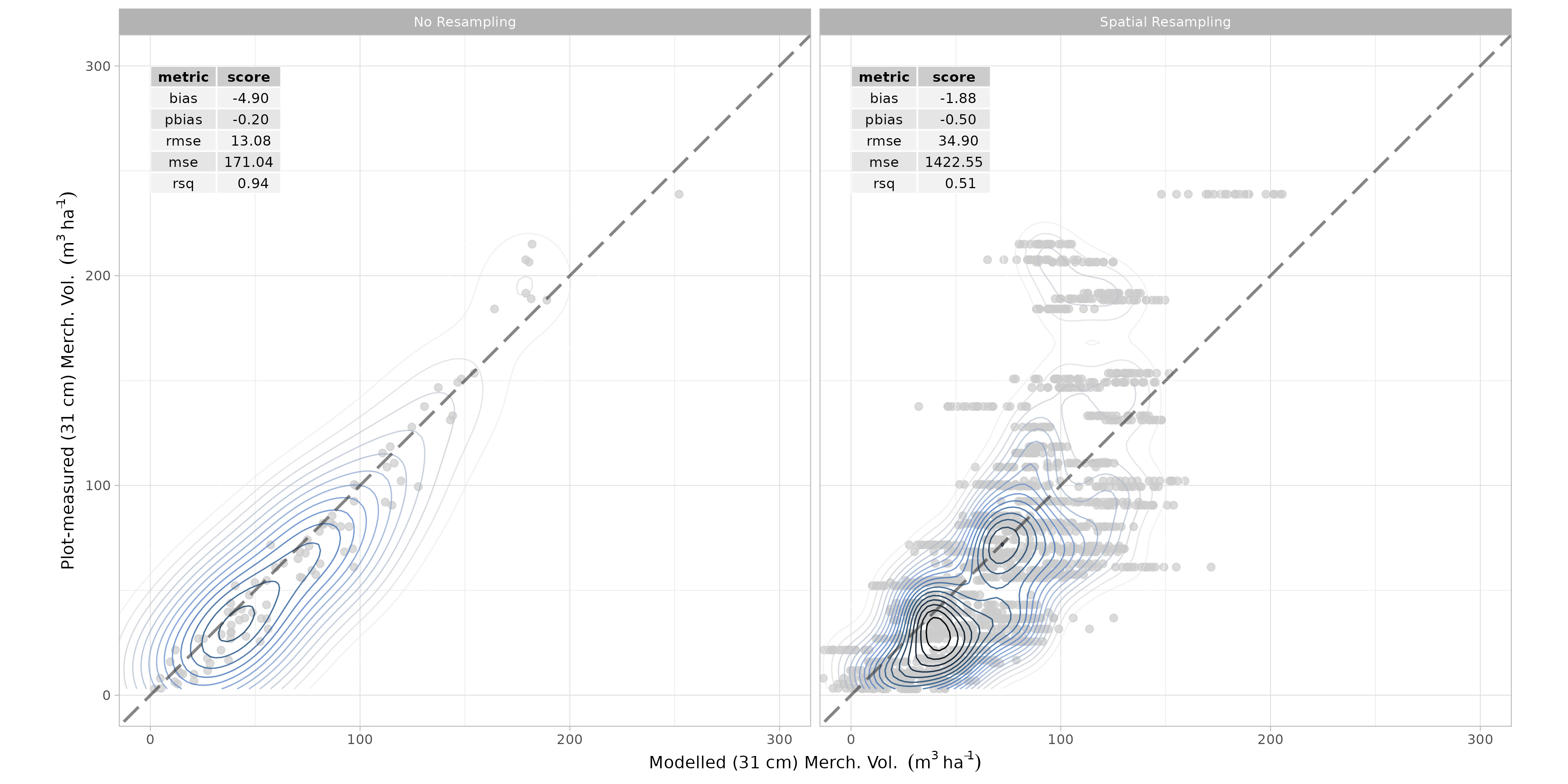
spatial resampling was once again carried out to evaluate model performance.
- Finally, the model was trained on the full forest plot inventory and predicted across the entire Kuamut area. Model predictions were cleaned by setting all predictions less than zero to zero and all predictions greater than 300 to NA.
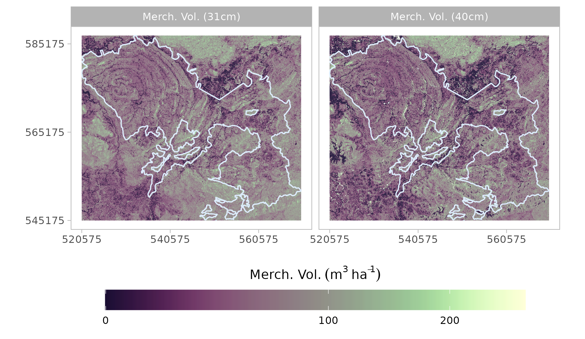
The previous steps including feature selection, ensemble model creation, resampling, model training and prediction were repeated for Merchantable Volume with cutting limits of 10 cm, 31 cm, and 40 cm.
7.5 Model Uncertainty
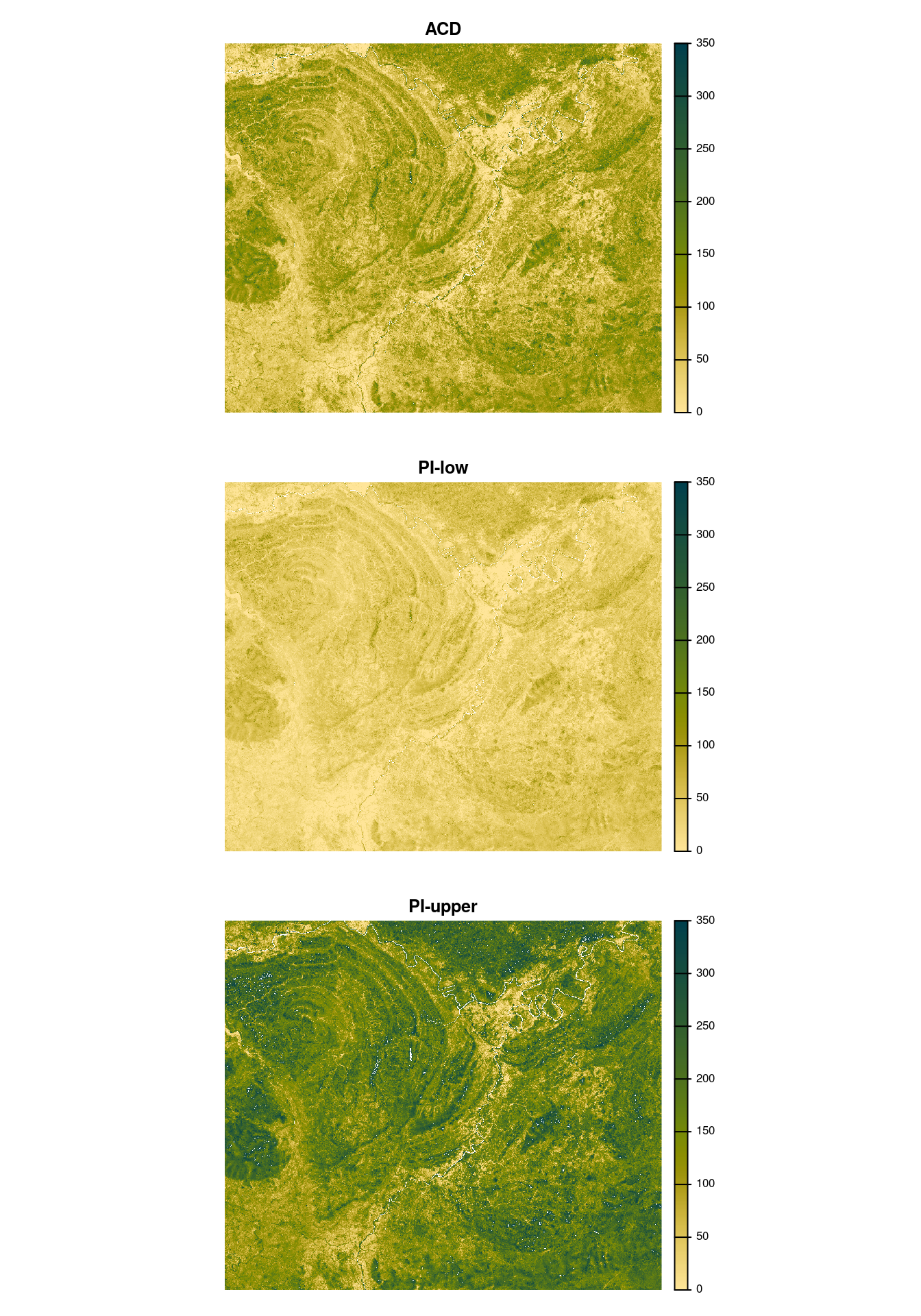
Prediction interval bands were generated for all volume and biomass raster maps. The first band in all maps is the prediction derived from the model, The second is the lower 2.5% Prediction Interval and the third is the 97.5% prediction interval.
Prediction intervals were generated as follows:
Bootstrap resampling of the tuned model was carried out with a total of 1000 iterations.
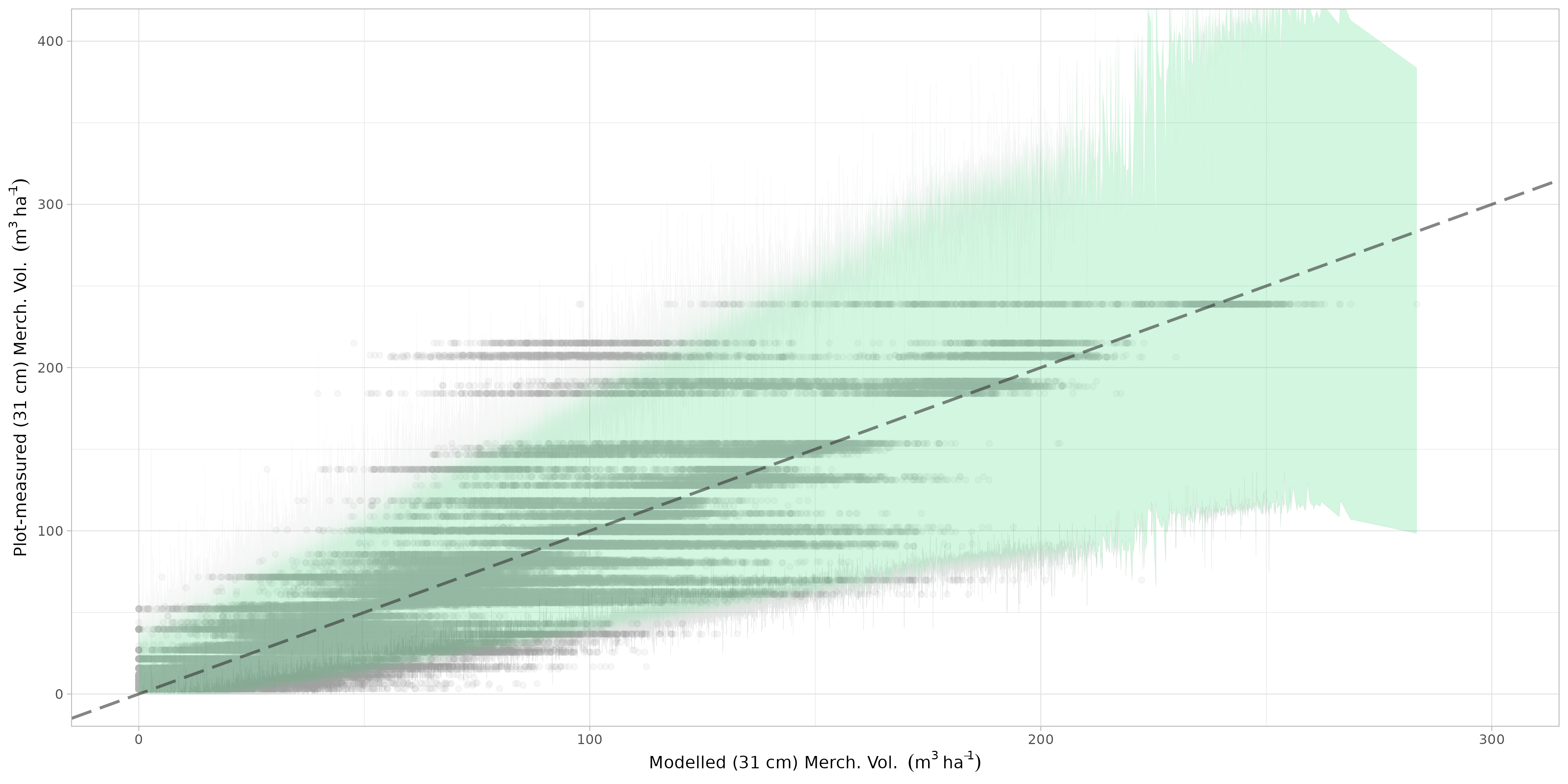
The bootstrapped predictions of the xgboost, svm models and the ensemble model, for all iterations,were aggregated. A quantile regression was fitted using xgboost and svm resamples as predictors and the ensemble model as response variable at both the 2.5 and 97.5 percentiles. The observed vs predicted plot for the quantile regression is presented in Figure 7.7.
- The Quantile regression models for the upper and lower prediction intervals were then used to predict the uncertainty spatially across the raster map. This required the generation of map bands for glm, xgboost and svm models before applying the two quantile regression models. An example of this spatial prediction for the three bands is shown below in Figure 7.8
These uncertainty bands are subsequently used in Chapter 18 to estimate the uncertainty of total timber volume estimates.