18 Baseline and Project Uncertainty
There are three key sources of potential uncertainty in the prediction of baseline and project based emissions. These include the total merchantable volume (TMV) stock for trees with a DBH > 31 cm and 40 cm and the observed growth rate of the project area (for each management strata).
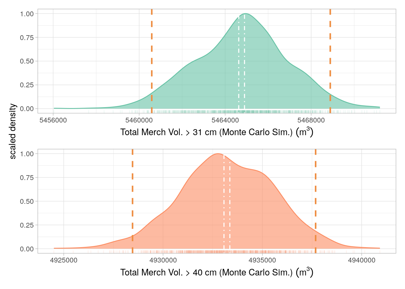
Uncertainty limits for TMV were derived as follows: Volume maps were masked to the project area, values from all three bands (mean, lower Prediction Interval (PI), upper PI) were converted to a dataframe. A simulation consisting of 10000 iterations was carried out, for each iteration, 100 random samples were drawn, for every cell, from a normal distribution, centered around the cell mean and constrained by the upper and lower 95% PI values. All cell values for every simulation (n= \(1e{+6}\)) were summed to give a simulated total; The 0.025th and 0.975th percentiles of the distribution were calculated and used as the PIs.
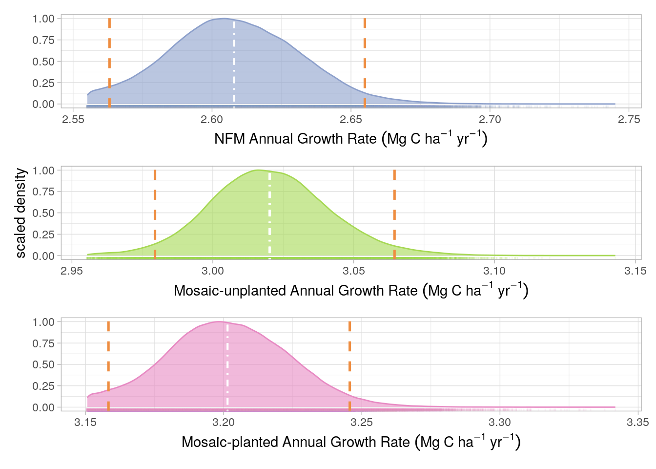
Uncertainty limits for the Project growth rate were derived from the fixed effects slopes of a linear mixed-effects (LME) model as described in Figure 17.2. Pixel ID was used as a random effect in the LME model and therefore we could generate a slope value, for each pixel, by summing the fixed effect (for the management strata intersecting the pixel) and the random effect. The distribution of these coefficients around the fixed effect value for each management strata was used to estimate growth rate uncertainty. Although the No-Go strata was included in the LMEM, it was not included in the uncertainty analysis because no credits are generated from the No-Go strata. As with the Volume uncertainty, the 0.025th and 0.975th percentiles of the slope coefficient distributions, for each management strata, were calculated and used as PIs
The uncertainty distributions and associated prediction intervals are presented, for the baseline estimates, in Figure 18.1 and, for the project scenario, in Figure 18.2 and Figure 18.3 for Monitoring Periods 1 and 2, respectively.
Growth rate uncertainty, Monitoring Report 1: 2016 - 2021
Growth rate uncertainty, Monitoring Report 2: 2022 - 2023
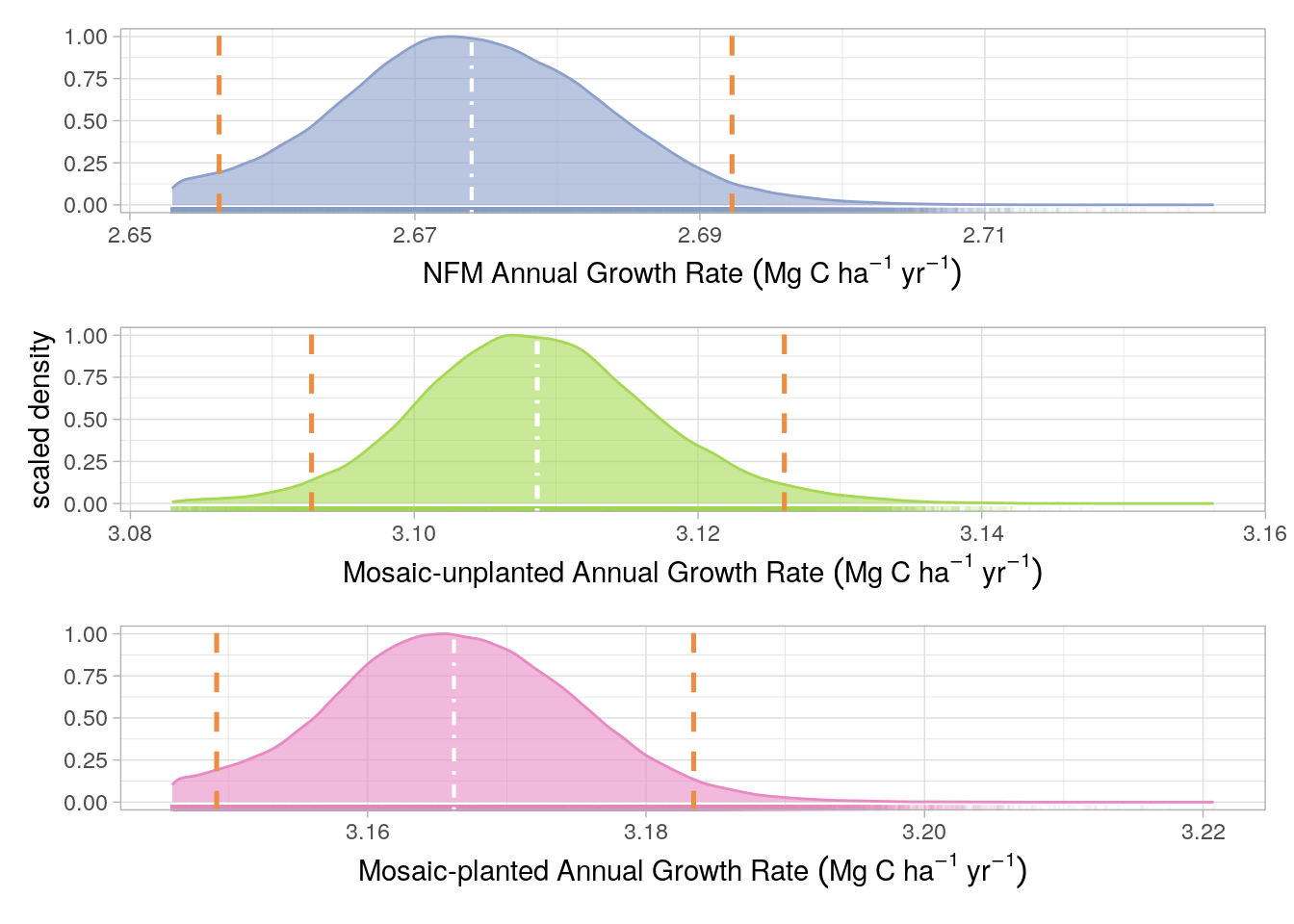
Although page 51 of the VM0010 methods, states that 95% confidence intervals (CIs) should be used to calculate uncertainty, we believe that prediction intervals (PIs) are a more appropriate error metric to adopt. We have made this decision for several reasons: (i) it is vastly more conservative (i.e returns wider confidence range) as shown in Figure 18.1 and Figure 18.3; (ii) PIs are arguably more appropriate for non parametric model estimates (as is the case for the machine learning-derived Merch. Vol. maps), and (iii) PIs are more informative about the true prediction uncertainty whereas will only inform on the confidence of the mean of a given distribution.
The uncertainty for all aforementioned error sources in Figure 18.1 and Figure 18.2 and Figure 18.3, for Monitoring periods 1 and 2, respectively, were calculated as in Equation 18.1: \[ U = \frac{PI_{upper}-PI_{lower}}{\mu} \cdot 100 \tag{18.1}\]
Where \(U\) is uncertainty, \(PI_{upper}\) is the upper 95% PI, \(PI_{lower}\) is the lower 95% PI and \(\mu\) is the mean derived from the model prediction (rather than the simulation). The predicted mean was used as this was more conservative than the simulated mean.
Verra define the quantification of uncertainty in Equation 42 of the VM0010 methods; we present this in Equation 18.2: \[ Utotal|ltpf = \sqrt{U^2_{|prj}+U^2_{|bsl}} \tag{18.2}\]
Where \(Utotal|ltpf\) is the total dimensionless uncertainty for the Logged to Protected Forest (LtPF) Project, \(U^2_{|prj}\) is the total dimensionless uncertainty for the improved forest management (IFM) activities in the project scenario, and \(U^2_{|bsl}\) is the total dimensionless uncertainty for the baseline scenario.
The Volume Map uncertainties encompass the uncertainty for the baseline scenario and the growth rate uncertainty captures the project-level IFM activity uncertainty.
We similarly combine all of these error sources, as indicated in Equation 18.2, but with the inclusion of each of the six potential error sources, as in shown in Equation 18.3: \[ Utotal|ltpf = \sqrt{U^2_{vol31}+U^2_{vol40}+U^2_{gr_{nfm}}+U^2_{gr_{mpl}}+U^2_{gr_{mun}}} \tag{18.3}\] Where \(U_{vol31}\) is the percent uncertainty for the total merchantable timber volume with a DBH > 31 cm, \(U_{vol40}\) is the percent uncertainty for the total merchantable timber volume with a DBH > 40 cm, \(U_{gr_{nfm}}\) is the percent uncertainty for the growth rate of the natural forest management (NFM) strata, \(U_{gr_{mpl}}\) is the percent uncertainty for the growth rate of the mosiac-planted management strata, and \(U_{gr_{mun}}\) is the percent uncertainty for the growth rate of the mosaic-unplanted management strata.
Section 8.4.1.1 of the VM0010 methods states that if \(Utotal|ltpf\) is less than 15%, then no deduction will result for uncertainty. For the Kuamut project, \(Utotal|ltpf\) is 5.3, 2%; therefore, no deduction was applied.
18.1 Code
Uncertainty Analysis Code R/uncertainty-analysis.R
#' Generates simulated values between the upper and lower limits from a normal
#' distribution based around the mean.
#'
#' @param .mean vector of means
#' @param .lower vector of lower prediction limits
#' @param .upper vector of upper prediction limits
#' @param .n How many values to create in the uniform distribution between lower and upper values.
#' @param .return_n How many values to draw from the uniform distribution based on normal distribution weighting.
#'
#' @return A vector of simulated cell means. i.e. between the upper and lower.
get_rand_from_norm <- Vectorize(
  function(.mean,
           .lower,
           .upper,
           .n = 1000,
           .return_n = 10) {
    if (all(c(.mean, .lower, .upper) == 0)) {
      return(rep(0, .return_n))
    }

    .dist <- runif(.n, .lower, .upper)

    sample(.dist,
      .return_n,
      replace = TRUE,
      prob = dnorm(.dist,
        mean = .mean,
        sd = sd(.dist),
        log = FALSE
      )
    )
  }
)


#' Wraps `get_rand_from_norm` to run multiple iterations in parallel. enables
#' multiple random draws for each iteration - increases mc efficiency.
#'
#' @param .mean vector of means
#' @param .lower vector of lower prediction limits
#' @param .upper vector of upper prediction limits
#' @param .n How many values to create in the uniform distribution between lower and upper values.
#' @param .return_n How many values to draw from the uniform distribution based on normal distribution weighting.
#' @param .reps How many times to repeat each iteration.
#' @param .seed the seed for reproducibility
#' @param .workers number of cores to run across - default is 50% of availabel cores
#' @param .progress should a progress bar be displayed?
#'
#' @return A vector of simulated volume totals.
#'
get_rand_from_norm_multi <- function(.mean,
                                     .lower,
                                     .upper,
                                     .n = 1000,
                                     .return_n = 100,
                                     .reps = 10,
                                     .seed = 5446,
                                     .workers = 5,
                                     .progress = FALSE) {
  wrap_it <- function(.iter) {
    DT <- get_rand_from_norm(
      .mean,
      .lower,
      .upper,
      .n,
      .return_n
    ) |>
      data.table::data.table() |>
      data.table::transpose()

    DT[, lapply(.SD, sum)] |>
      transpose()
  }

  future::plan(future::multisession, workers = .workers)
  sims <- furrr::future_map(1:.reps, wrap_it,
    .progress = .progress,
    .options = furrr_options(seed = .seed)
  ) |>
    data.table::rbindlist()
  future:::ClusterRegistry("stop")
  return(sims)
}

# just a wrapper for get_rand_from_norm_multi.
total_uncertainty <- function(x) {
  x <- as.data.frame(x)
  rand.sums.rep <- get_rand_from_norm_multi(x[[1]],
    x[[2]],
    x[[3]],
    .n = 1000,
    .return_n = 100,
    .reps = 10
  )
}


#' Create list of total volume uncertainty stats for plotting/reporting
#'
#' @param sim fthe results of the mc suimulation
#' @param ras the raster used to create the simulation. description
#'
#' @return a list of stats.
#'
sim_stats <- function(sim, ras) {
  true.sum <- sum(ras[[1]][], na.rm = TRUE)
  m <- mean(sim[[1]])
  ci <- confint(lm(sim[[1]] ~ 1))
  ci_p_error <- (ci[2] - ci[1]) / true.sum * 100

  pred_int <- quantile(sim[[1]], probs = c(0.025, 0.975))
  pi_p_error <- (pred_int[2] - pred_int[1]) / true.sum * 100

  list(
    true.sum = true.sum,
    sim.sum = m,
    ci = ci,
    ci_p_error = ci_p_error,
    pred_int = pred_int,
    pi_p_error = pi_p_error
  )
}


#' Create list of growth rate stats for plotting/reporting
#'
#' @param gr fixed effects slope values.
#'
#' @return a list of stats.
#'
gr_stats <- function(.gr) {
  m <- mean(.gr)
  ci <- confint(lm(.gr ~ 1))
  ci_p_error <- (ci[2] - ci[1]) / m * 100

  pred_int <- quantile(.gr, probs = c(0.025, 0.975))
  pi_p_error <- (pred_int[2] - pred_int[1]) / m * 100

  list(
    sim.sum = m,
    ci = ci,
    ci_p_error = ci_p_error,
    pred_int = pred_int,
    pi_p_error = pi_p_error
  )
}


#' function to plot uncertainty distributions.
#'
#' @param sim A data.table or vector with the simualted values.
#' @param sim.stat summary stats for the simulation (list)
#' @param .col a colour hex code
#' @param cutoff for merch vol sim labelling.
#' @param .lab turn on or off the y axis label.
#'
#' @return a ggplot object.
plot_sim <- function(
    sim, sim.stat, .col, cutoff = NULL,
    mgmt_strat = NULL, .lab = TRUE, .yvals = TRUE) {
  p <- data.frame(vals = sim) |>
    ggplot() +
    aes(x = vals) +
    geom_density(aes(y = after_stat(scaled)),
      fill = .col,
      col = .col, alpha = 0.6
    ) +
    geom_rug(colour = .col, alpha = 0.1) +
    geom_vline(aes(xintercept = sim.stat$ci[1]),
      linetype = 4,
      colour = "white", lwd = 0.6
    ) +
    geom_vline(aes(xintercept = sim.stat$ci[2]),
      linetype = 4,
      colour = "white", lwd = 0.6
    ) +
    geom_vline(aes(xintercept = sim.stat$pred_int[1]),
      linetype = 2,
      colour = "#EE8D41", lwd = 0.9
    ) +
    geom_vline(aes(xintercept = sim.stat$pred_int[2]),
      linetype = 2,
      colour = "#EE8D41", lwd = 0.9
    ) +
    theme_light()

  if (!is.null(cutoff)) {
    p <- p + labs(x = bquote(.(paste0(
      "Total Merch Vol. > ",
      cutoff, " (Monte Carlo Sim.)"
    )) ~ (m^3)))
  } else {
    p <- p + labs(x = bquote(
      .(paste0(mgmt_strat, " Annual Growth Rate")) ~ (Mg ~ C ~ ha^-1 ~ yr^-1)
    ))
  }

  if (isFALSE(.lab)) {
    p <- p + labs(y = "")
  } else {
    p <- p + labs(y = "scaled density")
  }

  if (isFALSE(.yvals)) {
    p <- p + ggplot2::theme(axis.text.y = ggplot2::element_blank())
  }

  return(p)
}

#' function to plot growth rate distributions.
#' stacks ggplot objects of the fixed effects of the growthrates for each strata
#' @param gr A list containing the fixed effect slopes from the biomass
#' growth model.
#' @param grs A list containing the summary stats for the growth rates.
#' @return a gpplot object.
growth_rate_stack_plot <- function(gr, grs) {
  plot_sim(gr["NFM"][[1]],
    grs["NFM"][[1]],
    mgmt_strat = "NFM",
    .col = "#8da0cb",
  ) /
    plot_sim(gr["Mosaic-unplanted"][[1]],
      grs["Mosaic-unplanted"][[1]],
      .col = "#a6d854",
      mgmt_strat = "Mosaic-unplanted"
    ) /
    plot_sim(gr["Mosaic-planted"][[1]],
      grs["Mosaic-planted"][[1]],
      .col = "#e78ac3",
      mgmt_strat = "Mosaic-planted"
    ) +
    patchwork::plot_layout(axes = "collect")
}


#' Main wrapper function for the uncertainty analysis target.
#'
#' @param aoi The project outline for clipping rasters
#' @param mv31 The merch. vol. raster for DHB > 31cm
#' @param mv40 The merch. vol. raster for DHB > 40cm
#' @param gr list of lists containing the fixed effect slopes from the biomass
#' growth model. nested list strucutre accomodates multiple monitoring periods.
#' @param fig.path default provided - the path to save the uncertianty plot image.
#'
#' @return a list with the calcuated uncertainty and plots/filepaths.
uncertainty_analysis <- function(aoi, mv31, mv40, gr,
                                 fig.path = set_path("Uncertainty-Analysis",
                                   parent = "data_out/MR_figures"
                                 )) {
  checkmate::assert_character(aoi)
  checkmate::assert_character(mv31)
  checkmate::assert_character(mv40)
  checkmate::assert_list(gr)
  checkmate::assert_character(fig.path)

  # read kuamut area
  ka <- vect(aoi)

  # mask 31cm vol raster by area
  vol31 <- rast(mv31) |>
    mask(ka)
  # mask 40cm vol raster by area
  vol40 <- rast(mv40) |>
    mask(ka)

  # convert per ha values to total per cell
  vol31.act <- vol31 * ((res(vol31)[1] * (res(vol31)[2])) / 10000)
  vol40.act <- vol40 * ((res(vol40)[1] * (res(vol40)[2])) / 10000)

  # run volume monte carlo analysis
  vol31.sim <- total_uncertainty(vol31.act)
  vol40.sim <- total_uncertainty(vol40.act)

  # Get MC stats -  prediction intervals etc.
  vol31.stats <- sim_stats(vol31.sim, vol31.act)
  vol40.stats <- sim_stats(vol40.sim, vol40.act)

  # get stats from growth rates

  names(gr) <- paste0("mr_", seq_along(gr))
  growth_rate_stats <- purrr::map(gr, \(x) purrr::map(x$fix_effs, gr_stats))

  # create plot.
  basline_unc_plot <-
    plot_sim(vol31.sim[[1]], vol31.stats,
      .col = "#66c2a5", "31 cm", .lab = TRUE
    ) /
    plot_sim(vol40.sim[[1]], vol40.stats,
      .col = "#fc8d62", "40 cm", .lab = TRUE
    ) +
    patchwork::plot_layout(axes = "collect")

  ggsave(paste0(fig.path, "-baseline.png"), basline_unc_plot)

  proj_unc_plots <- purrr::pmap(
    list(gr, growth_rate_stats),
    \(grvals, gr_stats) growth_rate_stack_plot(grvals$fix_effs, gr_stats)
  )

  proj_unc_plot_paths <- purrr::imap_chr(proj_unc_plots, \(x, y) {
    ppath <- paste0(fig.path, "-project-", y, ".png")
    ggsave(ppath, x, height = 15, width = 20, units = "cm")
    return(ppath)
  }) |>
    purrr::set_names(names(proj_unc_plots))


  # Combine Uncertainties with sum of squares.
  unc <- purrr::map_dbl(
    growth_rate_stats,
    ~ sum_of_squares(c(
      vol31.stats$pi_p_error,
      vol40.stats$pi_p_error,
      .x[["NFM"]]$pi_p_error,
      .x[["Mosaic-planted"]]$pi_p_error,
      .x[["Mosaic-unplanted"]]$pi_p_error
    ))
  )

  combined_unc_msg(unc)

  return(list(
    baseline_unc_plot = basline_unc_plot,
    proj_unc_plots = proj_unc_plots,
    baseline_plot_file = paste0(fig.path, "-baseline.png"),
    proj_plot_files = proj_unc_plot_paths,
    unc_plot_file = fig.path,
    uncertainty_val = unc
  ))
}

#' function to calculate the combined uncertainty. using the sum of squares.
#' @param uncs a vector of uncertainty values.
#' @return a single value of the combined uncertainty.
sum_of_squares <- function(uncs) {
  sqrt(sum(uncs^2))
}

#' useful messaging about the results of the uncertainty analysis.
#' @param unc_vec the vector of uncertainty values. (should be named)
#' @return NULL
combined_unc_msg <- function(unc_vec) {
  purrr::iwalk(
    unc_vec,
    \(.x, .y) {
      if (.x < 15) {
        cli::cli_alert_success(
          "Combined uncertainty estimates for {.y} = {round(.x, 3)}% (< 15%)"
        )
      } else {
        cli::cli_alert_danger(
          "Combined uncertainty estimates for {.y} = {round(.x, 3)}% (> 15%)"
        )
        cli::cli_warn(
          c(
            "x" = "Combined uncertainty estimates are above 15% for {.y}!",
            "!" = "You must inspect this in more detail!"
          )
        )
      }
    }
  )
  invisible()
}