17 Project Growth Rate Calculation
Project-level growth rate was calculated from the predicted ACD maps (Chapter 7) for each year of the monitoring period (2016-2022). By using the predicted ACD maps, as opposed to the plot measured ACD, we can mitigate any unforeseen bias introduced by the plot network distribution. This approach also enables us to robustly estimate growth rate across different management strata and in areas where no access was possible for field estimate. Incidentally, this analysis is demonstrated in Section 6.1 and is in line with the predictions derived in this chapter (Figure 17.2).
All annual ACD maps were inverse-masked for areas of deforestation detected in Chapter 16 and then masked by the project area, therefore excluding all cells that experienced any deforestation or that were outside of the project area. Then, the masked raster maps were converted to a single dataframe with the year value, management strata, and cell id as attributes.
Management Strata was considered in the model development because it was considered likely that the management strata, defined in the baseline, might reflect historic management practices and therefore influence the growth rate differentially across these strata. Further, it is indicated on page 89 of the VM0010 methods that only areas to be harvested should be considered for ongoing growth. The implication here is that growth rates for the management strata that we define as Inoperable/No-Go should be excluded from the growth rate calculation. However, rather than removing this NoGo strata from the raster data, as was done with deforested areas, the NoGo strata was included in the model as a fixed effect, allowing for its extraction from the model output.
17.1 Model Comparisons
In total, six different potential growth models were considered as shown in Table 17.2. Two linear models were tested, one of which simply considered the year as a predictor (model 6 in Table 17.2) and another that considered the year and management strata, as an interaction term (model 5). It was considered necessary to test the inclusion of pixel ID as a random effect in order to account for spatial autocorrelation and local variation in growth rates. Therefore, four linear mixed-effects models (LMEM) were tested; one with a random effect of pixel ID only (model 4), one with year as a random slope and pixel id as a random effect (model 3), models 2 and 1 were the same as model 4 and model 3 respectively, but with the addition of management strata as a fixed effect.
Of these three models, The LMEM with management strata as an interactive fixed effect and year and pixel ID as random slopes/effects, reported the lowest Akaike Information Criterion (AIC) and Bayesian Information Criterion (BIC) values. Furthermore, this model form more appropriately represents ecological processes by accounting for fine-scale spatial variation in growth rates and captures the variability across management strata which likely results from variation in historic logging activity, in response to slope and accessibility.
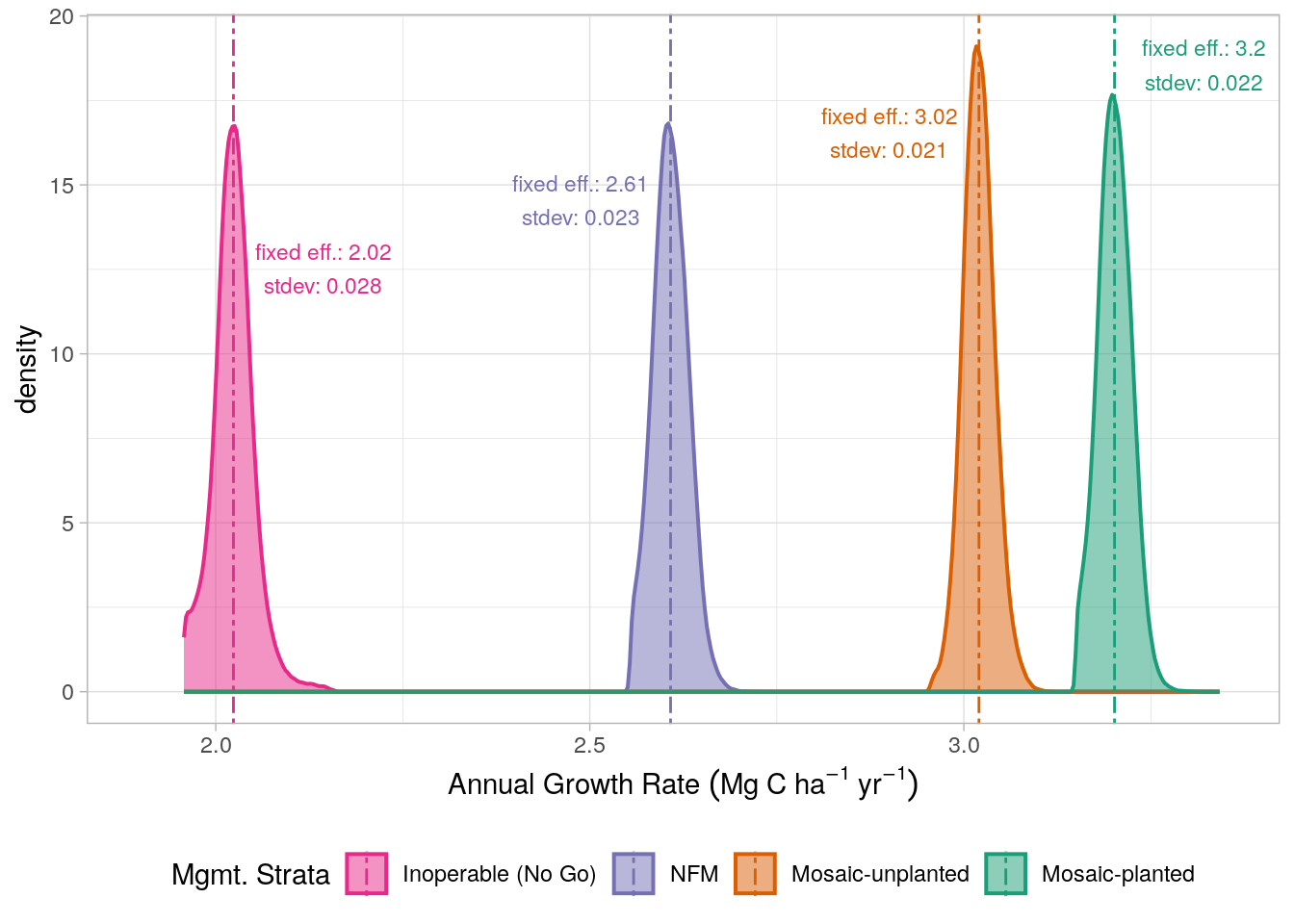
Growth model results, Monitoring Report 1: 2016 - 2021
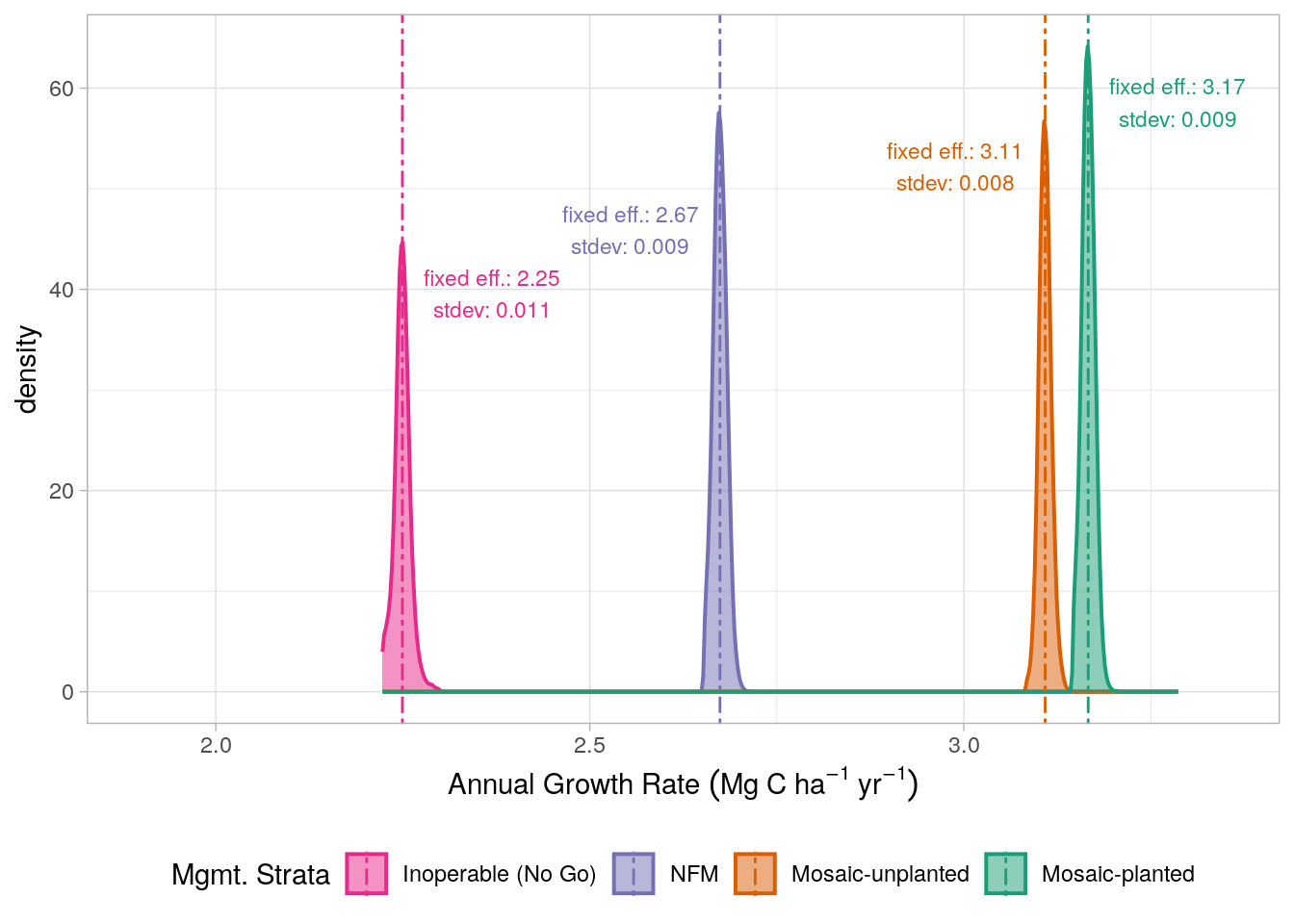
Growth model results, Monitoring Report 2: 2022 - 2023
We therefore selected model 1 in Table 17.2 as our final model. The fixed effects of the model were extracted and the slope values for each level of the management strata were used to define growth rate. Before applying these growth rates for the final ERR calculations in Chapter 21, the strata-level species conservation factors (as calculated in Chapter 10) were discounted from the growth rates. The resulting “adjusted” growth rates are presented in Table 17.4.
To determine the variability in growth rates, for each strata, we extracted the model’s random effects (for each pixel that intersected the relevant strata) and added the fixed effect slope, providing model coefficients defining growth for each pixel in the project area. The distribution of these slope coefficients are presented in Figure 17.2. These distributions also enable us to make estimates of the uncertainty in growth rates across the project area for each strata; this is demonstrated in Chapter 18 (Figure 18.3).
The extent to which these growth rates reflect the historic forest management practices for the project area is noteworthy. The steeper areas and those that are not allowed to be logged due to their proximity to the rivers/roads (NFM and No-Go) display notably lower growth rates relative to the lower gradient areas (i.e. mosaic management) where historic logging activity is likely to have been more intensive. Of the planted and non-planted mosaic management strata, the planted regions, which are characterised by their lower gradient display higher growth rates, likely reflecting the greater levels of historic disturbance in these areas.
17.2 Code
Project biomass growth rate code R/proj-growth-rate-multi.R
#' @title Create Management strata Raster
#' @description Create a raster of the management strata.
#' @param cols A vector of mgmt strata to include in the raster.
#' @param .mgmt_strat The management strata sf object.
#' @param .aoi The AOI sf object.
#' @param .deforest The deforestation sf object.
#' @param .ras_template The raster template to use to rasterize the mgmt strata.
#' @return A raster of the management strata.
mgmt_ras <- function(cols, .mgmt_strat, .aoi, .deforest, .ras_template) {
  terra::rasterize(
    .mgmt_strat[.mgmt_strat$mgmt_strata %in% cols, ],
    terra::rast(.ras_template),
    field = "mgmt_strata",
    touches = TRUE
  ) |>
    terra::mask(.aoi) |>
    terra::mask(.deforest, inverse = TRUE)
}

#' @title Create ACD time series dataframe
#' @description Create a dataframe of the ACD time series for each pixel.
#' @param r.p The raster of ACD for a given year.
#' @param .y The name of the raster.
#' @param .kaoi The AOI sf object.
#' @param .deforest The deforestation sf object.
#' @param .mgmt_strat_ras The raster of the management strata.
#' @return A dataframe of the ACD raster for each pixel.
create_acd_df <- function(r.p, .y, .kaoi, .deforest, .mgmt_strat_ras) {
  .year <- as.numeric(gsub(".*?([0-9]+).*", "\\1", .y))
  agb <- terra::rast(r.p) |>
    terra::mask(.kaoi) |>
    terra::mask(.deforest, inverse = TRUE)
  dt <- c(agb, .mgmt_strat_ras) |>
    as.data.frame(xy = TRUE) |>
    data.table::setDT()

  dt[, YEAR := .year]
  dt[, pix_id := paste0(x, "_", y)]
  return(dt)
}

#' @title Plot the fixed effects
#' @description Plot the fixed effects.
#' @param slopes_df A dataframe of the fixed effects long format.
#' @param slope_stats_df A dataframe of the fixed effects stats.
#' @return A ggplot object.
fix_effects_plot <- function(
    slopes_df, slope_stats_df,
    fig_path) {
  p <- slopes_df |>
    ggplot() +
    aes(x = slope, fill = mgmt_strata, colour = mgmt_strata) +
    geom_density(linewidth = 0.7, alpha = 0.5) + #
    scale_fill_brewer(palette = "Dark2", direction = -1) +
    scale_colour_brewer(palette = "Dark2", direction = -1) +
    geom_vline(slope_stats_df,
      mapping = aes(xintercept = fix_eff, colour = mgmt_strata),
      linetype = 6,
      linewidth = 0.5
    )

  built_plot <- ggplot2::ggplot_build(p)
  # Extract the y-axis limits
  y_max <- built_plot$layout$panel_params[[1]]$y.range[2]

  p <- p +
    geom_text(slope_stats_df,
      mapping = aes(
        label = paste0("fixed eff.: ", round(fix_eff, 2)),
        x = fix_eff + c(0.12, -0.12, 0.12, -0.12),
        y = c(0.95, 0.85, 0.65, 0.75) * y_max,
        colour = mgmt_strata
      ),
      size = 3, show.legend = FALSE
    ) +
    geom_text(slope_stats_df,
      mapping = aes(
        label = paste0("stdev: ", round(stdev, 3)),
        x = fix_eff + c(0.12, -0.12, 0.12, -0.12),
        y = c(0.9, 0.8, 0.6, 0.7) * y_max,
        colour = mgmt_strata
      ),
      size = 3, show.legend = FALSE
    ) +
    labs(
      x = bquote("Annual Growth Rate" ~ (Mg ~ C ~ ha^-1 ~ yr^-1)),
      fill = "Mgmt. Strata", colour = "Mgmt. Strata", y = "density"
    ) +
    theme_light() +
    coord_cartesian(xlim = c(1.9, 3.35))

  ggsave(fig_path, p, width = 9, height = 4)

  return(list(
    bio_gr_ggplot = p,
    bio_gr_ggplot_path = fig_path
  ))
}


#' @title Calculate Biomass growth rate
#' @description Calculate the biomass growth rate for each mgmt strata.
#' @param agb_rasters A list of rasters containing the AGB for each year.
#' @param aoi_path The path to the AOI spatial vector.
#' @param deforest_path The path to the deforestation spatial vector.
#' @param mgmt_strat_path The path to the management strata spatial vector.
#' @param fig_path The path to the output figure.
#' @param workers The number of workers to use for parallel processing.
#' @return A list containing the fixed effects, growth rates, and a
#' ggplot object.
calculate_proj_growth <- function(
    agb_rasters,
    aoi_path,
    deforest_path,
    mgmt_strat_path,
    workers = 6) {
  # define the parralel backend
  future::plan("multisession", workers = workers)

  # read in spatial objects
  mgmt_strat <- terra::vect(mgmt_strat_path)
  deforest <- terra::vect(deforest_path)
  kaoi <- terra::vect(aoi_path)

  # create raster of management strata
  mgmt_strat_ras1 <- mgmt_ras(
    c("NFMCoupesGo", "MosaicPLANT", "MosaicUNplanted", "NoGo"),
    .mgmt_strat = mgmt_strat,
    .aoi = kaoi,
    .deforest = deforest,
    .ras_template = agb_rasters[[1]]
  )

  # create dataframe of the ACD time series for each pixel
  ACD_ts <- purrr::imap(
    agb_rasters,
    ~ create_acd_df(.x, .y, kaoi, deforest, mgmt_strat_ras1)
  ) |>
    data.table::rbindlist()

  ACD_ts[, mgmt_strata := relevel(ACD_ts$mgmt_strata, "NoGo")] # set top level

  # save ACD_ts as rds for use in parallel processing to avoid memory issues
  # resulting from passing large objects to each worker.
  temp_rds <- tempfile(fileext = ".rds")
  saveRDS(ACD_ts, temp_rds)

  # function to fit a model and return AIC and BIC
  fit_mod <- function(form, mixed = FALSE, REML = FALSE) {
    df <- readRDS(temp_rds)
    if (isFALSE(mixed)) {
      mod <- lm(form, data = df)
      form_chr <- paste0("lm(", Reduce(paste, deparse(form)), ")")
    } else {
      mod <- lme4::lmer(form,
        REML = REML,
        data = df,
        na.action = na.omit
      )
      form_chr <- paste0("lmer(", Reduce(paste, deparse(form)), ")")
    }

    tibble::tibble(
      model = form_chr,
      AIC = AIC(mod),
      BIC = BIC(mod)
    )
  }

  # list of formulas to test
  formulas <- list(
    formula(ACD_mgC_ha ~ YEAR),
    formula(ACD_mgC_ha ~ YEAR * mgmt_strata),
    formula(ACD_mgC_ha ~ YEAR + (1 | pix_id)),
    formula(ACD_mgC_ha ~ YEAR * mgmt_strata + (1 | pix_id)),
    formula(ACD_mgC_ha ~ YEAR + (1 + YEAR | pix_id)),
    formula(ACD_mgC_ha ~ YEAR * mgmt_strata + (1 + YEAR | pix_id))
  )
  # list of booleans indicating whether the model is mixed or not
  mix_list <- c(FALSE, FALSE, TRUE, TRUE, TRUE, TRUE)

  # create a model performance table of the tested models
  mod_perf_tab <- furrr::future_map2(
    formulas,
    mix_list,
    fit_mod
  ) |>
    dplyr::bind_rows() |>
    dplyr::arrange(AIC)


  # create lookup for mgmt strata based on pix_id
  pix_id_lookup <- ACD_ts[, .(mgmt_strata = unique(mgmt_strata)), by = pix_id]

  # fit the best model
  mod <- lme4::lmer(
    ACD_mgC_ha ~ YEAR * mgmt_strata + (1 + YEAR | pix_id),
    REML = TRUE,
    data = ACD_ts,
    na.action = na.omit
  )

  # get fixed effects of the mem - used as growth rate
  fe <- lme4::fixef(mod)

  #' function to unname the fixed effects
  unname_fe <- function(x) {
    unname(fe[x])
  }
  # create vector of growth rates for annual calcs
  gr_vec <- c(
    "Inoperable (No Go)" = unname_fe("YEAR"),
    "NFM" = unname_fe("YEAR") + unname_fe("YEAR:mgmt_strataNFMCoupesGo"),
    "Mosaic-planted" =
      unname_fe("YEAR") + unname_fe("YEAR:mgmt_strataMosaicPLANT"),
    "Mosaic-unplanted" =
      unname_fe("YEAR") + unname_fe("YEAR:mgmt_strataMosaicUNplanted")
  )

  # Create a lookup table
  rename_lookup <- data.table(
    old_value = c(
      "NFMCoupesGo", "MosaicPLANT", "MosaicUNplanted", "NoGo"
    ),
    new_value = c(
      "NFM", "Mosaic-planted", "Mosaic-unplanted", "Inoperable (No Go)"
    )
  )

  # get random effects of the mem to estimate variance around growth rates
  ran_effs <- lme4::ranef(mod, condVar = FALSE)$pix_id |>
    data.table::setDT(keep.rownames = TRUE) |>
    data.table::setnames("rn", "pix_id") |>
    merge(pix_id_lookup, by = "pix_id", all.x = TRUE)

  # rename the mgmt strata
  ran_effs[rename_lookup, mgmt_strata := new_value,
    on = .(mgmt_strata = old_value)
  ]
  ran_effs[, mgmt_strata := factor(mgmt_strata, levels = c(
    "Inoperable (No Go)", "NFM", "Mosaic-unplanted", "Mosaic-planted"
  ))]

  # add the fixed effects based on mgmt strata
  ran_effs[, slope := YEAR + gr_vec[match(mgmt_strata, names(gr_vec))]]

  # split the fixed effects into a list for uncertainty analysis
  slopes_list <- split(ran_effs$slope, ran_effs$mgmt_strata)

  # create stat df for plotting
  stat_df <- ran_effs[, .(stdev = sd(slope)), by = mgmt_strata]
  stat_df[, fix_eff := gr_vec[match(mgmt_strata, names(gr_vec))]]
  stat_df[, mgmt_strata := factor(mgmt_strata, levels = c(
    "Inoperable (No Go)", "NFM", "Mosaic-unplanted", "Mosaic-planted"
  ))]

  return(list(
    fix_effs = slopes_list,
    fix_effs_long = ran_effs,
    growth_rates = gr_vec,
    mod_perform_tab = mod_perf_tab,
    growth_stats = stat_df
  ))
}