12 Natural Forest Management (NFM) Timber Harvest Plan
As in Chapter 11, this chapter also outlines the proposed baseline harvest plan but for NFM coupes. The key difference for the NFM coupes is that the cutting limit is 40 cm DBM and therefore, the 40 cm Merchantable Volume map is used to extract harvestable volume in this case.
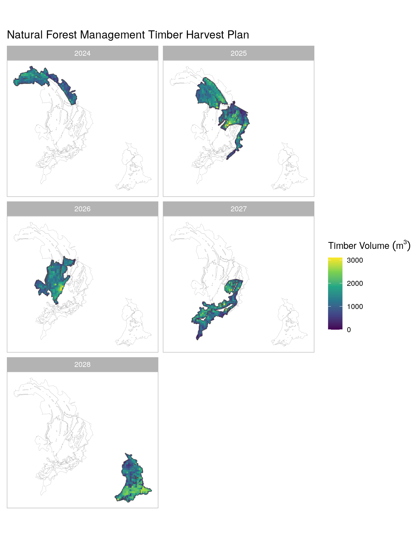
The following map depicts the spatial sequencing of the baseline timber harvest plan for the NFM strata. Note that the baseline for NFM strata begins in 2024.
12.1 Code
NFM Timber Harvest Plan Code R/TimberHarvestPlan_NFM_Coupes.R
#' NFM Timber Harvest Plan
#'
#' @description This function creates the timber harvest plan for the NFM
#' Plantings coupes.
#'
#' @param boundary_src path to the boundary polygon
#' @param NFMCoupes_src path to the NFMCoupes spatial polygon
#' @param dbh40_src path to the 31cm DBH Merchantable Volume raster
#' @param dbh10_src path to the 10cm DBH Merchantable Volume raster
#' @param acd_src path to the Above Ground Carbon (ACD) raster
#' @param setup logging plot setup size in hectares (31ha was average in
#' INFAPRO area see Philipon 2020)
#' @param ReEntry default is 10. Re-entry logging in number of years
#' @param R2ReEntry default is 15. Second round of Re-entry logging in number
#' of years
#' @param sp_conserve_factor derived from `R/protected-trees-stats.R`
#' @return A list containg the following: parcel_csv_list: a table containing
#' the parcel-level data, nfm_src: a gridded coupes dataset for NFM,
#' nfm_ggplots: a ggplot object with a map of the harvest plan, nfm_vol31_spv:
#' A spatial vector containing the timber volume data.
timber_harvest_plan_NFM <- function(boundary_src, NFMCoupes_src,
                                    dbh40_src, dbh10_src, acd_src,
                                    setup = 31, ReEntry = 10, R2ReEntry = 15,
                                    sp_conserve_factor) {
  # init values...
  ha <- (100 * 100) # 1 hectare is 100m x 100m
  setup_SqM <- setup * ha # gives size in square meters
  ploty <- sqrt(setup_SqM)
  plotx <- ploty

  Boundary <- sf::read_sf(boundary_src)


  ## Area for Improved Forest Management
  NFMCoupes <- sf::read_sf(NFMCoupes_src) |>
    mutate(
      BLOCK_N = case_when(
        is.na(BLOCK_N) ~ "SE_heal",
        TRUE ~ BLOCK_N
      ),
      YearEnd = case_when(
        YearEnd == 0 ~ max(YearEnd),
        TRUE ~ YearEnd
      )
    )

  # Run separately for three raster options (40cm cutting limit for NFM NFM),
  # 10cm (all for residual damage), and ACD for comparison
  fileName_list <- list(
    "40cmDBH" = dbh40_src,
    "10cmDBH" = dbh10_src,
    "ACD_10cm" = acd_src
  )

  # Convert Rasters from volume/ha to absolute volume per cell.
  # function in : 'R/coupes_helpers.R'
  abs_vol_list <- fileName_list |>
    purrr::imap(~ create_abs_volume(.x, .y, Boundary, NFMCoupes))

  create_NFM_grid <- function(strata, type_name, out_path) {
    RentryYear <- max(as.integer(strata$YearEnd)) + ReEntry

    # Make the grid of individual setups to be logged
    grid <- sf::st_make_grid(strata, cellsize = c(plotx, ploty))

    gridmask <- sf::st_intersection(grid, strata)

    # join attribute tables
    strata_grid <- sf::st_join(
      sf::st_as_sf(gridmask),
      sf::st_as_sf(strata),
      join = sf::st_intersects, largest = TRUE
    )

    strata_grid_poly <- sf::st_collection_extract(
      x = strata_grid,
      type = "POLYGON"
    )
    strata_grid <- strata_grid_poly |>
      mutate(id = row_number()) |>
      mutate(
        LogYear = case_when(
          BLOCK_N %in% c("YL3/04", "YS2/09") ~ RentryYear,
          BLOCK_N %in% c("YS4/04", "YS3/09", "YL4/03(2)") ~ RentryYear + 1,
          BLOCK_N %in% c("YS4/05(2)") ~ RentryYear + 2,
          BLOCK_N %in% c("YL4/03(1)", "YS4/05(1)", "YT1/06(I)")
          ~ RentryYear + 3,
          BLOCK_N %in% c("YLH5/06(A)", "YLH5/06(B)", "YLH1/08", "SE_heal")
          ~ RentryYear + 4,
          TRUE ~ -9999
        ),
        area_ha = units::set_units(
          sf::st_area(strata_grid_poly),
          value = hectare
        )
      ) |>
      select(!Area_ha) # dropping old area column.

    if (nrow(strata_grid |> dplyr::filter(LogYear == -9999)) > 0) {
      stop("Check the Block Names!")
    }

    region_list <- list(gridmask, strata, strata_grid)

    areas <- purrr::map_dbl(region_list, ~ get_areas(.x))
    purrr::walk(areas, ~ testthat::expect_equal(.x, areas[1]))

    sf::write_sf(strata_grid, out_path, delete_dsn = TRUE)

    return(strata_grid)
  }

  NFM_polygon_out_dir <- dirname(NFMCoupes_src)
  NFM_polygon_out_shp <- file.path(
    NFM_polygon_out_dir, "NFMCoupes_THP_Grid.shp"
  )
  NFM_grid <- create_NFM_grid(
    strata = NFMCoupes, type_name = "NFM-PLANTED",
    out_path = NFM_polygon_out_shp
  )

  # extract values for strata
  # function in : 'R/coupes_helpers.R'
  NFM_strat_ext <- purrr::map(.x = abs_vol_list, ~ extract_strata(.x, NFM_grid))

  # make plots for each logging year
  nfm_ggplots <- purrr::imap(
    .x = NFM_strat_ext,
    ~ plot_setups(.x, .y, "NFM-PLANTED", outline_width = 0.6)
  )


  ParcelsIntoFuture <- purrr::imap(
    .x = NFM_strat_ext,
    ~ summarise_parcels_nfm(.x, .y,
      sp_conserve_factor =
        sp_conserve_factor,
      R2ReEntry = R2ReEntry
    )
  )

  parcel_csv_list <- purrr::imap(
    ParcelsIntoFuture,
    ~ save_parcels(.x, .y, "NFM_THP_Parcels")
  )

  return(c(
    parcel_csv_list,
    list(nfm_src = NFM_polygon_out_shp),
    list(nfm_ggplots = nfm_ggplots),
    list(nfm_vol31_spv = NFM_strat_ext$`40cmDBH`)
  ))
}
Additional Timber Harvest Plan Functions R/coupes_helpers.R
#' convert raster density to absolute values.
#'
#' @param ras_src raster source relative to data folder
#' @param ras_name the desired name of the raster
#' @param aoi the area of interest (spatial polygon or sf)
#' @param overlay coupes areas for plot vis
#' @param scale.factor default is 10000 i.e number of square meters in a ha.
#'
#' @return raster with absolute values.
#' @details
#' This function converts the raster density values to absolute values.
#' The raster density values are per hectare, so we need to convert them to
#' absolute values. The scale factor is the number of square meters in a
#' hectare.
#'
create_abs_volume <- function(
    ras_src, ras_name, aoi, overlay, scale.factor = 1e4) {
  V_BSL <- terra::rast(ras_src)[[1]]
  V_BSL * ((terra::res(V_BSL)[1] * terra::res(V_BSL)[2]) / scale.factor)
}


#' Extract sum
#'
#' Simple function to extract sum of raster within coupes.
#'
#' @param V_BSLpPix a raster object. Either Timber Volume or ACD.
#' @param strata_grid a gridded spatial vector of the strata of interest. sf object.
#'
#' @return sf object with sum of V_BSL per setup.
#' @details
#' extract sum of V_BSL per setup using MosaicGrid ( will be == V_EX when back
#' to per ha) UNITS should be sum per pixel
extract_strata <- function(V_BSLpPix, strata_grid) {
  strata_grid |>
    mutate(VolSum = exactextractr::exact_extract(
      V_BSLpPix, strata_grid, "sum"
    )) # use {exactextractr} for speed.
}


#' plot ACD or Timber Volume
#'
#' @param setups
#' @param dbh
#' @param mosaic_type
#' @param outline_width
#'
#' @return ggplot object.
plot_setups <- function(setups, dbh, mosaic_type, outline_width = 0.03, .ncol = 2) {
  p <- setups |>
    ggplot() +
    aes(fill = VolSum) +
    geom_sf(
      data = sf::st_geometry(dplyr::summarise(setups)), colour = "grey70", fill = "transparent",
      inherit.aes = FALSE, lwd = 0.1
    ) +
    geom_sf(data = setups, colour = "grey30", fill = "transparent", lwd = outline_width) +
    geom_sf(colour = NA) +
    scale_fill_viridis_c() +
    theme_light() +
    facet_wrap(~LogYear, ncol = .ncol) +
    labs(title = dbh) +
    theme(
      axis.title.x = element_blank(),
      axis.text.x = element_blank(),
      axis.ticks.x = element_blank(),
      axis.title.y = element_blank(),
      axis.text.y = element_blank(),
      axis.ticks.y = element_blank(),
      panel.grid.major = element_blank(),
      panel.grid.minor = element_blank()
    )
}


#' save parcel csv
#'
#' @param parcel_df the parcel summary df to save.
#' @param dbh one of: c("ACD_10cm", "40cmDBH", "31cmDBH", "10cmDBH")
#' @param save_pref character prefix for the file path
#'
#' @return file path (character) of the saved csv.
save_parcels <- function(parcel_df, dbh, save_pref) {
  # Save Parcels using 30cm DBH, 10cm DBH (or ACD as a check)
  if (dbh != "ACD_10cm") {
    what <- paste0("V_EX_", dbh)
  } else {
    what <- dbh
  }
  # Save each of the three Parcel files to csv

  parcels_save_path <- set_path(paste0(
    "RoutputProducts/",
    save_pref,
    what, ".csv"
  ))
  write.table(parcel_df, parcels_save_path)

  return(parcels_save_path)
}


#' helper function for initial parcel defs
#'
#' @param setups
#'
#' @return sf object of summarised parcels.
parcel_setup <- function(setups, dbh) {
  Parc1 <- setups |>
    group_by(LogYear) |>
    dplyr::summarise(VolSum = sum(VolSum, na.rm = TRUE))
  Parc <- Parc1 |>
    mutate(Area_ha = units::set_units(sf::st_area(Parc1), ha)) |>
    sf::st_drop_geometry()

  # For Asner Map version ACD, for merchantable, name is V_EX
  if (dbh == "ACD_10cm") {
    Parc <- mutate(Parc, ACD = round(VolSum / as.numeric(Area_ha)))
  } else {
    Parc <- mutate(Parc, V_EX = round(VolSum / as.numeric(Area_ha))) # -> V_EX
  }
  return(Parc)
}

#' function to create mosaic parcels
#'
#' @param setups
#' @param dbh
#' @param Coupe_planted
#'
#' @return sf object of summarised parcels.
summarise_parcels_mos <- function(setups, dbh, Coupe_planted = TRUE,
                                  sp_conserve_factor, Yrs2Plant, Rotation,
                                  P_ha) {
  ### Here we add up the volume of all setups into the yearly parcels.
  Parcels <- parcel_setup(setups, dbh)

  # In the Mosaics we will assume a baseline of extracting only 70% of all
  # merchantable timber this is a more conservative way to account for species
  # that shouldn't be logged.

  if (dbh == "31cmDBH") {
    #  # Don't extract all merchantable volume based on sp_conserve_factor
    Parcels <- mutate(Parcels, V_EX = round(V_EX * sp_conserve_factor, 1))
  }
  strata_def <- function(plant_type) {
    paste("Mosaic", plant_type, sep = "-")
  }
  Parcels <- Parcels |>
    mutate(
      Strata = case_when(
        isTRUE(Coupe_planted) ~ strata_def("planted"),
        TRUE ~ strata_def("unplanted")
      ),
      Plant = case_when(
        isTRUE(Coupe_planted) ~ "planted",
        TRUE ~ "unplanted"
      ),
      Rotation = "First"
    )

  #------------ Future rounds of logging ------------------------------------
  # For transparency and simplicity We keep predictions for Future logging
  # periods as straightforward as possible as these will be revisited
  #-------------------------------------------------------------------------#
  ## Modelling overall growth rate based on planting rate and rotation
  plantingArea <- as.numeric(P_ha)
  AReaPlantPA <- round(plantingArea / Yrs2Plant)

  ParcelsNextRotation <- data.frame(
    LogYear = seq(from = (2017 + Rotation), length.out = Yrs2Plant),
    VolSum = rep(NA, length.out = Yrs2Plant),
    Area_ha = rep(AReaPlantPA, length.out = Yrs2Plant),
    V_EX = rep(95 * sp_conserve_factor, length.out = Yrs2Plant),
    Strata = paste("Mosaic-planted"),
    Plant = paste("planted"),
    Rotation = paste("Second")
  ) |>
    mutate(VolSum = Area_ha * V_EX)

  # colname for ACD carbon map check
  if (dbh == "ACD_10cm") {
    colnames(ParcelsNextRotation)[4] <- "ACD"
  }

  # If the area is planted, there will be a future rotation
  # (according to above), if not planted, then not during this baseline period
  if (isTRUE(Coupe_planted)) {
    return(rbind(Parcels, ParcelsNextRotation))
  } else {
    return(Parcels)
  }
}


#' Function to create Natural Forest Management Parcels.
#'
#' @param setups
#' @param dbh
#'
#' @return sf object of summarised parcels.
summarise_parcels_nfm <- function(setups, dbh, sp_conserve_factor, R2ReEntry) {
  Parcels <- parcel_setup(setups, dbh)

  # In # the NFM we will assume a baseline of extracting only 70% of all
  # merchantable timber. This is a more conservative way to account for
  # species that shouldn't be logged and would fit with 'selective logging'.

  if (dbh == "40cmDBH") {
    # Don't extract all merchantable volume based on sp_conserve_factor
    Parcels <- mutate(Parcels, V_EX = round(V_EX * sp_conserve_factor, 1))
  }

  Parcels$Strata <- "NFM"
  Parcels$Plant <- "unplanted"
  Parcels$Rotation <- "First"

  # Future rounds of logging:
  # For transparency and simplicity We keep predictions for Future logging
  # periods as straightforward as possible as these will be revisited
  ParcelsNextRentry <- Parcels |>
    mutate(
      LogYear = LogYear + R2ReEntry,
      Rotation = "Second"
    )

  # given we have a conservative baseline extraction rate, we estimate the same
  # volume could and would be extracted after a further 15 years
  rbind(Parcels, ParcelsNextRentry)
}